Cube Example - Basic Usage

In this tutorial you will learn the basic usage of EncoderMap with a little toy data set.

Run this notebook on Google Colab:

Find the documentation of EncoderMap:

https://ag-peter.github.io/encodermap

For Google colab only:

If you’re on Google colab, please uncomment these lines and install EncoderMap.

# !wget https://raw.githubusercontent.com/AG-Peter/encodermap/main/tutorials/install_encodermap_google_colab.sh
# !sudo bash install_encodermap_google_colab.sh

Import Libraries

Before we can get started using EncoderMap we first need to import the EncoderMap library:

import encodermap as em

2023-02-07 11:06:04.369263: I tensorflow/core/platform/cpu_feature_guard.cc:193] This TensorFlow binary is optimized with oneAPI Deep Neural Network Library (oneDNN) to use the following CPU instructions in performance-critical operations:  AVX2 AVX512F FMA
To enable them in other operations, rebuild TensorFlow with the appropriate compiler flags.
2023-02-07 11:06:04.531537: W tensorflow/compiler/xla/stream_executor/platform/default/dso_loader.cc:64] Could not load dynamic library 'libcudart.so.11.0'; dlerror: libcudart.so.11.0: cannot open shared object file: No such file or directory; LD_LIBRARY_PATH: /opt/hostedtoolcache/Python/3.9.16/x64/lib
2023-02-07 11:06:04.531563: I tensorflow/compiler/xla/stream_executor/cuda/cudart_stub.cc:29] Ignore above cudart dlerror if you do not have a GPU set up on your machine.
2023-02-07 11:06:05.380515: W tensorflow/compiler/xla/stream_executor/platform/default/dso_loader.cc:64] Could not load dynamic library 'libnvinfer.so.7'; dlerror: libnvinfer.so.7: cannot open shared object file: No such file or directory; LD_LIBRARY_PATH: /opt/hostedtoolcache/Python/3.9.16/x64/lib
2023-02-07 11:06:05.380614: W tensorflow/compiler/xla/stream_executor/platform/default/dso_loader.cc:64] Could not load dynamic library 'libnvinfer_plugin.so.7'; dlerror: libnvinfer_plugin.so.7: cannot open shared object file: No such file or directory; LD_LIBRARY_PATH: /opt/hostedtoolcache/Python/3.9.16/x64/lib
2023-02-07 11:06:05.380625: W tensorflow/compiler/tf2tensorrt/utils/py_utils.cc:38] TF-TRT Warning: Cannot dlopen some TensorRT libraries. If you would like to use Nvidia GPU with TensorRT, please make sure the missing libraries mentioned above are installed properly.

We will also need some aditional imports for plotting:

import matplotlib.pyplot as plt
from mpl_toolkits.mplot3d import Axes3D
%matplotlib inline

To ensure that this notebook yields reproducible output, we fix the randomness in tensorflow.

import tensorflow as tf
tf.random.set_seed(3)

Load Data

Next, we need to load our data. EncoderMap expects the input data to be a 2d array. Each line should contain one data point and the number of columns is the dimensionality of the data set. Here, you could load data from any source. In this tutorial, however, we will use a function to generate a toy data set. The function random_on_cube_edges distributes a given number of points randomly on the edges of a cube. We can also add some Gaussian noise by specifying a sigma value.

high_d_data, ids = em.misc.create_n_cube()

let’s look at the data we have just created:

print("high_d_data\n", high_d_data, '\n')
print("ids\n", ids)

high_d_data
 [[-0.01487527 -0.07052302 -0.05676328]
 [-0.02696381  0.00161324  0.02731435]
 [ 0.09265312  0.02985699  0.11462655]
 ...
 [ 0.98327783  0.97677343  1.02679615]
 [ 0.94078978  1.00286322  0.99799477]
 [ 1.0234299   0.96051847  0.99450113]]

ids
 [ 1.  1.  1. ... 11. 11. 11.]

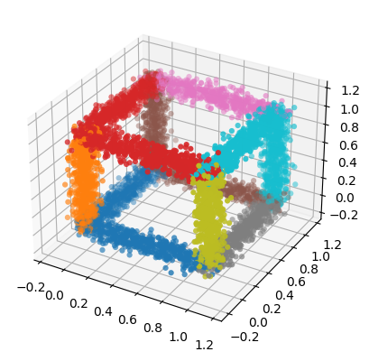
high_d_data is a 2d array where each row represents one point in a 3d space. ids contains a number form 0 to 11 for each point. This number tells us which edge of the cube each point belongs to. We can use these ids to color the points in a plot. The following code creates a scatter plot of the data:

fig = plt.figure()
ax = fig.add_subplot(111, projection='3d')
ax.scatter(high_d_data[:, 0], high_d_data[:, 1], high_d_data[:, 2],
            c=ids, marker="o", linewidths=0, cmap="tab10")

<mpl_toolkits.mplot3d.art3d.Path3DCollection at 0x7f0ae8aa7e20>

Select Parameters

Now that we have loaded our data we need to select parameters for EncoderMap. Parameters are stored in an object derived from the Parameters class. A list of the available parameters can be found here. We do not need to bother with all these parameters, as the default parameters should be fine in many cases. We should, however adjust some parameters for this example:

The seed parameters will fix the random states of tensorflow and numpy. Make sure to not set this parameter when you train your networks.

parameters = em.Parameters(
main_path = em.misc.run_path("runs/cube"),
periodicity = float("inf"),
n_steps = 200,
checkpoint_step = 100,
seed = 2
)

The main_path defines where output files will be written. run_path is a helper function which creates a new numbered run directory. When you call this for the first time it will create a directory runs/cube/run0. If this directory already exist it will instead create the directory runs/cube/run1 and so forth.

The periodicity is important for periodic input such as angular values. As the input in this case in not periodic we set the periodicity to infinite.

n_steps defines the number of training iterations.

Furthermore, we should adjust the sigmoid functions applied to the high-dimensional and low-dimensional pairwise distances of the distance based part of the cost function. There a three parameters for each sigmoid which should be given in the following order:

(sig_h, a_h, b_h, sig_l, a_l, b_l)

In order to select these parameters it is helpful to plot the sigmoid functions together with a histogram of the pairwise distances in the data set.

parameters.dist_sig_parameters = (0.3, 6, 6, 1, 4, 6)
em.plot.distance_histogram(high_d_data,
                           parameters.periodicity,
                           parameters.dist_sig_parameters,
                           bins=50)

(<AxesSubplot: title={'center': 'high-d'}, xlabel='distance'>,
 <AxesSubplot: >,
 <AxesSubplot: title={'center': 'low-d'}, xlabel='distance'>)

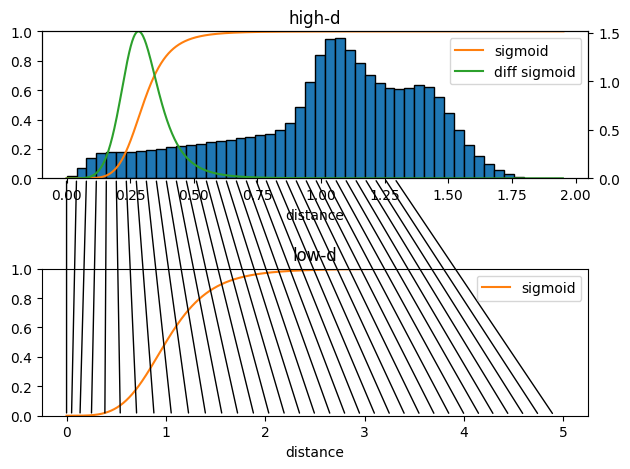
The upper plot shows the high-d sigmoid function and the pairwise distances histogram, the plot also shows the derivative of the sigmoid function. This derivative shows the sensitive range of the distance based part of the cost function. As it is not possible to preserve all pairwise distances in the low-d representation we want to tune this sensitive range to match distances which are most important for us. Usually very short distances are not important for the structure of a data set as these distances stem from points inside the same local region. Long distances might be interesting but can hardly be reproduced in a lower dimensional representation. Somewhere in between are the most important distances which contain the information how local regions in the data are connected to neighboring regions.

The lower plot shows the low-d sigmoid function. The black lines connecting the plots of the high-d sigmoid and the low-d sigmoid indicate to which low-dimensional distances high-dimensional distences will ideally be mapped with your choice of sigmoid parameters.

The sigmoid parameters for the low-d space can be selected according to the following rules:

sig_l = 1 (is irrelevant as it only scales the low-dimensional map)

a_l = a_h * n_dimensions_l / n_dimensions_h

b_l= b_h

Further information about the the selection of these sigmoid parameters can be found in the Sketchmap literature.

Feel free to play with different sigmoid parameters and see how the sigmoid function changes in the previous cell. I recommend to continue the tutorial with (0.3, 6, 6, 1, 4, 6) for a start but you can come back later and changes these parameters.

Get more info about parameters

To get more information from your parameters use the .parameters attribute.

print(parameters.parameters)

    Parameter            | Value                    | Description
    ---------------------+--------------------------+---------------------------------------------------
    n_neurons            | [128, 128, 2]            | List containing number of neurons for each layer
                         |                          | up to the bottleneck layer. For example [128, 128,
                         |                          | 2] stands for an autoencoder with the following
                         |                          | architecture {i, 128, 128, 2, 128, 128, i} where i
                         |                          | is the number of dimensions of the input data.
                         |                          | These are Input/Output Layers that are not
                         |                          | trained.
    ---------------------+--------------------------+---------------------------------------------------
    activation_functions | ['', 'tanh', 'tanh', ''] | List of activation function names as implemented
                         |                          | in TensorFlow. For example: "relu", "tanh",
                         |                          | "sigmoid" or "" to use no activation function. The
                         |                          | encoder part of the network takes the activation
                         |                          | functions from the list starting with the second
                         |                          | element. The decoder part of the network takes the
                         |                          | activation functions in reversed order starting
                         |                          | with the second element form the back. For example
                         |                          | ["", "relu", "tanh", ""] would result in a
                         |                          | autoencoder with {"relu", "tanh", "", "tanh",
                         |                          | "relu", ""} as sequence of activation functions.
    ---------------------+--------------------------+---------------------------------------------------
    periodicity          | inf                      | Defines the distance between periodic walls for
                         |                          | the inputs. For example 2pi for angular values in
                         |                          | radians. All periodic data processed by EncoderMap
                         |                          | must be wrapped to one periodic window. E.g. data
                         |                          | with 2pi periodicity may contain values from -pi
                         |                          | to pi or from 0 to 2pi. Set the periodicity to
                         |                          | float("inf") for non-periodic inputs.
    ---------------------+--------------------------+---------------------------------------------------
    learning_rate        | 0.001                    | Learning rate used by the optimizer.
    ---------------------+--------------------------+---------------------------------------------------
    n_steps              | 200                      | Number of training steps.
    ---------------------+--------------------------+---------------------------------------------------
    batch_size           | 256                      | Number of training points used in each training
                         |                          | step
    ---------------------+--------------------------+---------------------------------------------------
    summary_step         | 10                       | A summary for TensorBoard is writen every
                         |                          | summary_step steps.
    ---------------------+--------------------------+---------------------------------------------------
    checkpoint_step      | 100                      | A checkpoint is writen every checkpoint_step
                         |                          | steps.
    ---------------------+--------------------------+---------------------------------------------------
    dist_sig_parameters  | (0.3, 6, 6, 1, 4, 6)     | Parameters for the sigmoid functions applied to
                         |                          | the high- and low-dimensional distances in the
                         |                          | following order (sig_h, a_h, b_h, sig_l, a_l, b_l)
    ---------------------+--------------------------+---------------------------------------------------
    distance_cost_scale  | 500                      | Adjusts how much the distance based metric is
                         |                          | weighted in the cost function.
    ---------------------+--------------------------+---------------------------------------------------
    auto_cost_scale      | 1                        | Adjusts how much the autoencoding cost is weighted
                         |                          | in the cost function.
    ---------------------+--------------------------+---------------------------------------------------
    auto_cost_variant    | mean_abs                 | defines how the auto cost is calculated. Must be
                         |                          | one of: * `mean_square` * `mean_abs` * `mean_norm`
    ---------------------+--------------------------+---------------------------------------------------
    center_cost_scale    | 0.0001                   | Adjusts how much the centering cost is weighted in
                         |                          | the cost function.
    ---------------------+--------------------------+---------------------------------------------------
    l2_reg_constant      | 0.001                    | Adjusts how much the L2 regularisation is weighted
                         |                          | in the cost function.
    ---------------------+--------------------------+---------------------------------------------------
    gpu_memory_fraction  |                          | Specifies the fraction of gpu memory blocked. If
                         |                          | set to 0, memory is allocated as needed.
    ---------------------+--------------------------+---------------------------------------------------
    analysis_path        |                          | A path that can be used to store analysis
    ---------------------+--------------------------+---------------------------------------------------
    id                   |                          | Can be any name for the run. Might be useful for
                         |                          | example for specific analysis for different data
                         |                          | sets.
    ---------------------+--------------------------+---------------------------------------------------
    model_api            | sequential               | A string defining the API to be used to build the
                         |                          | keras model. Defaults to `sequntial`. Possible
                         |                          | strings are: * `functional` will use keras'
                         |                          | functional API. * `sequential` will define a keras
                         |                          | Model, containing two other models with the
                         |                          | Sequential API. These two models are encoder and
                         |                          | decoder. * `custom` will create a custom Model
                         |                          | where even the layers are custom.
    ---------------------+--------------------------+---------------------------------------------------
    loss                 | emap_cost                | A string defining the loss function. Defaults to
                         |                          | `emap_cost`. Possible losses are: *
                         |                          | `reconstruction_loss` will try to train output ==
                         |                          | input * `mse`: Returns a mean squared error loss.
                         |                          | * `emap_cost` is the EncoderMap loss function.
                         |                          | Depending on the class `Autoencoder`, `Encodermap,
                         |                          | `ACDAutoencoder`, different contributions are used
                         |                          | for a combined loss. Autoencoder uses atuo_cost,
                         |                          | reg_cost, center_cost. EncoderMap class adds
                         |                          | sigmoid_loss.
    ---------------------+--------------------------+---------------------------------------------------
    training             | auto                     | A string defining what kind of training is
                         |                          | performed when autoencoder.train() is callsed. *
                         |                          | `auto` does a regular model.compile() and
                         |                          | model.fit() procedure. * `custom` uses gradient
                         |                          | tape and calculates losses and gradients manually.
    ---------------------+--------------------------+---------------------------------------------------
    batched              | True                     | Whether the dataset is batched or not.
    ---------------------+--------------------------+---------------------------------------------------
    tensorboard          |                          | Whether to print tensorboard information. Defaults
                         |                          | to False.
    ---------------------+--------------------------+---------------------------------------------------
    seed                 | 2                        | Fixes the state of all operations using random

Performe Dimensionality Reduction

Now that we have set up the parameters and loaded the data, it is very simple to performe the dimensionality reduction. All we need to do is to create an EncoderMap object and call its train method. The EncoderMap object takes care of setting up the neural network autoencoder and once you call the train method this network is trained to minimize the cost function as specified in the parameters.

e_map = em.EncoderMap(parameters, high_d_data)
e_map.train()

Output files are saved to runs/cube/run0 as defined in 'main_path' in the parameters.

2023-02-07 11:06:17.290503: W tensorflow/compiler/xla/stream_executor/platform/default/dso_loader.cc:64] Could not load dynamic library 'libcuda.so.1'; dlerror: libcuda.so.1: cannot open shared object file: No such file or directory; LD_LIBRARY_PATH: /opt/hostedtoolcache/Python/3.9.16/x64/lib
2023-02-07 11:06:17.290549: W tensorflow/compiler/xla/stream_executor/cuda/cuda_driver.cc:265] failed call to cuInit: UNKNOWN ERROR (303)
2023-02-07 11:06:17.290575: I tensorflow/compiler/xla/stream_executor/cuda/cuda_diagnostics.cc:156] kernel driver does not appear to be running on this host (fv-az267-630): /proc/driver/nvidia/version does not exist
2023-02-07 11:06:17.291547: I tensorflow/core/platform/cpu_feature_guard.cc:193] This TensorFlow binary is optimized with oneAPI Deep Neural Network Library (oneDNN) to use the following CPU instructions in performance-critical operations:  AVX2 AVX512F FMA
To enable them in other operations, rebuild TensorFlow with the appropriate compiler flags.
 50%|████▉     | 99/200 [00:04<00:01, 67.67it/s, Loss after step 100=5.78]WARNING:absl:Function `_wrapped_model` contains input name(s) Encoder_0_input with unsupported characters which will be renamed to encoder_0_input in the SavedModel.
WARNING:absl:Function `_wrapped_model` contains input name(s) Decoder_0_input with unsupported characters which will be renamed to decoder_0_input in the SavedModel.
100%|█████████▉| 199/200 [00:07<00:00, 71.92it/s, Loss after step 200=4.9] WARNING:absl:Function `_wrapped_model` contains input name(s) Encoder_0_input with unsupported characters which will be renamed to encoder_0_input in the SavedModel.
WARNING:absl:Function `_wrapped_model` contains input name(s) Decoder_0_input with unsupported characters which will be renamed to decoder_0_input in the SavedModel.
100%|██████████| 200/200 [00:08<00:00, 24.03it/s, Loss after step 200=4.9]
WARNING:absl:Function `_wrapped_model` contains input name(s) Encoder_0_input with unsupported characters which will be renamed to encoder_0_input in the SavedModel.
WARNING:absl:Function `_wrapped_model` contains input name(s) Decoder_0_input with unsupported characters which will be renamed to decoder_0_input in the SavedModel.

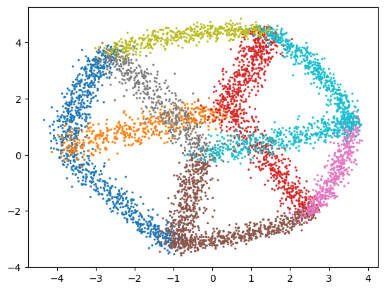
Once the network is trained we can feed high dimensional data into the encoder part of the network and read the values from the bottleneck layer. That is how we project data to the low dimensional space. The following line projects all our high-dimensional data to the low-dimensional space:

low_d_projection = e_map.encode(high_d_data)

Let’s have a look at the result and plot the data:

fig, ax = plt.subplots()
ax.scatter(low_d_projection[:, 0], low_d_projection[:, 1], c=ids, s=5, marker="o", linewidths=0, cmap="tab10")
plt.show()

Generate High-Dimensional Data

We can not only use the encoder part of the network to project points the to the low-dimensional space. Also, the inverse procedure is possible using the decoder part of the Network. This allows to project any point from the low-dimensional space to the high dimensional space.

In the following we feed all low-dimension points into the decoder part of the network to generate high dimensional points:

generated = e_map.generate(low_d_projection)

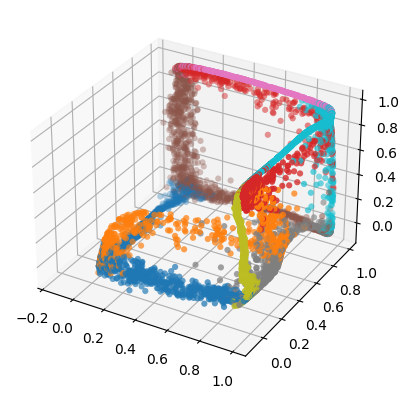
Let’s have a look at these generated point:

fig = plt.figure()
ax = fig.add_subplot(111, projection='3d')
ax.scatter(generated[:, 0], generated[:, 1], generated[:, 2], c=ids, marker="o", linewidths=0, cmap="tab10")
plt.show()

You probable see again a cube like structure. The reconstruction, however, will not be perfect, as information is lost when the data is projected to a lower dimensional space.

Conclusion

In this tutorial you have learned how to set parameters, run the dimensionality reduction and how to project points from the high-dimensional space to the low dimensional space and vice versa.