Customize EncoderMap: Logging Custom Scalars

Welcome

Welcome to the customization part of the EncoderMap tutorials. EncoderMap was redesigned from the ground up using the great customizability of the TensorFlow library. In the new version of EncoderMap all objects can be changed, adjusted by the user or even reused in other TensorFlow projects. The notebooks in this section help you in customizing EnocderMap and adding custom functionality.

This notebook specifically helps you in logging custom scalars to TensorBoard to visualize additional data during the training of EncoderMap’s networks on your data and help you investigate the problems at hand.

Run this notebook on Google Colab:

Find the documentation of EncoderMap:

https://ag-peter.github.io/encodermap

Goals

In this tutorial you will learn:

• How to subclass EncoderMap’s ``EncoderMapBaseMetric` to add additonal logging capability to TensorBoard <#subclass>`__

• Use the ``y_true` and y_pred parmeters in the update() function <#y_pred>`__

For Google colab only:

If you’re on Google colab, please uncomment these lines and install EncoderMap.

# !wget https://gist.githubusercontent.com/kevinsawade/deda578a3c6f26640ae905a3557e4ed1/raw/b7403a37710cb881839186da96d4d117e50abf36/install_encodermap_google_colab.sh
# !sudo bash install_encodermap_google_colab.sh

If you’re on Google Colab, you also want to download the data we will use:

# !wget https://raw.githubusercontent.com/AG-Peter/encodermap/main/tutorials/notebooks_starter/asp7.csv

Import libraries

before we can start exploring how to add custom data to TensorBoard, we need to import some libraries.

import encodermap as em
import tensorflow as tf
import numpy as np
import pandas as pd
import plotly.graph_objects as go

%load_ext autoreload
%autoreload 2

/home/kevin/git/encoder_map_private/encodermap/__init__.py:194: GPUsAreDisabledWarning: EncoderMap disables the GPU per default because most tensorflow code runs with a higher compatibility when the GPU is disabled. If you want to enable GPUs manually, set the environment variable 'ENCODERMAP_ENABLE_GPU' to 'True' before importing EncoderMap. To do this in python you can run:

import os; os.environ['ENCODERMAP_ENABLE_GPU'] = 'True'

before importing encodermap.
  _warnings.warn(

Adding custom scalars to TensorBoard by subclassing EncoderMapBaseMetric

EncoderMap has implemented a EncoderMapBaseMetric class, that can be used to implement such features. It can be found in the callbacks submodule in EncoderMap

?em.callbacks.EncoderMapBaseMetric

We will subclass EncoderMapBaseMetric to add additional logging capabilities to our training. As a first example, we will just log a random-normal value. For that we create our own Metric class. We only need to implement a single method, called update. Normally this method gets the input of the network as the y_true argument and the output as the y_pred argument (remember. EncoderMap is a regression task and so the y_true values do not stem from training data, but are the input data, that the network tries to regress against). However, in our case we won’t need these values, as we just take samples from a random normal distribution. Here, it is best to use the builtin tensorflow function tf.random.normal(), with the NumPy function np.random.normal, the random state will not be updated and the output will be constant (rather than random).

To log the random value, we also need to use tf.summary.scalar()

class RandomNormalMetric(em.callbacks.EncoderMapBaseMetric):
    def update(self, y_true, y_pred):
        r = tf.random.normal(shape=(1, ))[0]
        tf.summary.scalar("my random metric", r)
        return r

This metric can easily be added to a EncoderMap instance via the add_metric() method.

p = em.Parameters(n_steps=1_000, tensorboard=True)
emap = em.EncoderMap(parameters=p)
emap.add_metric(RandomNormalMetric)
history = emap.train()

Output files are saved to /home/kevin/git/encoder_map_private/docs/source/notebooks/customization_nb as defined in 'main_path' in the parameters.
Saved a text-summary of the model and an image in /home/kevin/git/encoder_map_private/docs/source/notebooks/customization_nb, as specified in 'main_path' in the parameters.

100%|█████████████████████| 1000/1000 [00:11<00:00, 88.24it/s, Loss after step 1000=0.598]

Saving the model to /home/kevin/git/encoder_map_private/docs/source/notebooks/customization_nb/saved_model_2024-12-29T13:13:56+01:00.keras. Use `em.EncoderMap.from_checkpoint('/home/kevin/git/encoder_map_private/docs/source/notebooks/customization_nb')` to load the most recent model, or `em.EncoderMap.from_checkpoint('/home/kevin/git/encoder_map_private/docs/source/notebooks/customization_nb/saved_model_2024-12-29T13:13:56+01:00.keras')` to load the model with specific weights..
This model has a subclassed encoder, which can be loaded independently. Use `tf.keras.load_model('/home/kevin/git/encoder_map_private/docs/source/notebooks/customization_nb/saved_model_2024-12-29T13:13:56+01:00_encoder.keras')` to load only this model.
This model has a subclassed decoder, which can be loaded independently. Use `tf.keras.load_model('/home/kevin/git/encoder_map_private/docs/source/notebooks/customization_nb/saved_model_2024-12-29T13:13:56+01:00_decoder.keras')` to load only this model.

Our custom metric will be available in the 'RandomNormalMetric Metric' key of the history.

fig = go.Figure(
    data=[
        go.Histogram(x=history.history["RandomNormalMetric Metric"], nbinsx=20)
    ]
)
fig.show()

In tensorboard, the custom scalar can be found in the Scalars section:

Use the y_true and y_pred parameters in the update() function

To get a feel how these parameters can be used, when subclassing an EncoderMapBaseMetric, we will have a look at one of EncoderMap’s cost functions. The auto cost compares the input and output pairwise distances. In EncoderMap, there are three variants of doing so:

1. mean_square: The mean_square variant is computed via:

auto_cost = tf.reduce_mean(tf.square(y_true - y_pred))

2. mean_abs: The mean_abs variant is computed via:

auto_cost = tf.reduce_mean(tf.abs(y_true - y_pred))

3. mean_norm: The mean_norm variant is computed via:

auto_cost = tf.reduce_mean(tf.norm(y_true - y_pred))

However, during training only one of these variants will be emplyed. Let’s write some metrics, that will calculate the cost variants regardless of which variant is actually used during training. For that, we will create three new em.callbacks.EncoderMapBaseMetric subclasses:

class MeanSquare(em.callbacks.EncoderMapBaseMetric):
    def update(self, y_true, y_pred):
        c = tf.reduce_mean(tf.square(y_true - y_pred))
        tf.summary.scalar("mean square", c)
        return c


class MeanAbs(em.callbacks.EncoderMapBaseMetric):
    def update(self, y_true, y_pred):
        c = tf.reduce_mean(tf.abs(y_true - y_pred))
        tf.summary.scalar("mean abs", c)
        return c


class MeanNorm(em.callbacks.EncoderMapBaseMetric):
    def update(self, y_true, y_pred):
        c = tf.reduce_mean(tf.norm(y_true - y_pred))
        tf.summary.scalar("mean norm", c)
        return c

We will also add a new metric which logs the maximum value of the y_true value.

class MaxVal(em.callbacks.EncoderMapBaseMetric):
    def update(self, y_true, y_pred):
        c = tf.reduce_max(y_true)
        tf.summary.scalar("mean norm", c)
        return c

With these new metrics, we can train another instance of the EncoderMap network.

p = em.Parameters(n_steps=1_000, tensorboard=True)
emap = em.EncoderMap(parameters=p)
emap.add_metric(MeanSquare)
emap.add_metric(MeanAbs)
emap.add_metric(MeanNorm)
emap.add_metric(MaxVal)
history = emap.train()

Output files are saved to /home/kevin/git/encoder_map_private/docs/source/notebooks/customization_nb as defined in 'main_path' in the parameters.
Saved a text-summary of the model and an image in /home/kevin/git/encoder_map_private/docs/source/notebooks/customization_nb, as specified in 'main_path' in the parameters.

100%|█████████████████████| 1000/1000 [00:13<00:00, 72.47it/s, Loss after step 1000=0.567]

Saving the model to /home/kevin/git/encoder_map_private/docs/source/notebooks/customization_nb/saved_model_2024-12-29T13:14:11+01:00.keras. Use `em.EncoderMap.from_checkpoint('/home/kevin/git/encoder_map_private/docs/source/notebooks/customization_nb')` to load the most recent model, or `em.EncoderMap.from_checkpoint('/home/kevin/git/encoder_map_private/docs/source/notebooks/customization_nb/saved_model_2024-12-29T13:14:11+01:00.keras')` to load the model with specific weights..
This model has a subclassed encoder, which can be loaded independently. Use `tf.keras.load_model('/home/kevin/git/encoder_map_private/docs/source/notebooks/customization_nb/saved_model_2024-12-29T13:14:11+01:00_encoder.keras')` to load only this model.
This model has a subclassed decoder, which can be loaded independently. Use `tf.keras.load_model('/home/kevin/git/encoder_map_private/docs/source/notebooks/customization_nb/saved_model_2024-12-29T13:14:11+01:00_decoder.keras')` to load only this model.

And have a look at how these metrics compare:

from plotly.subplots import make_subplots

fig = make_subplots(rows=2, cols=1)

fig.add_trace(
    go.Scatter(
        y=history.history["MeanSquare Metric"],
        mode="lines",
        name="mean square",
    ),
    col=1,
    row=1,
)
fig.add_trace(
    go.Scatter(
        y=history.history["MeanAbs Metric"],
        mode="lines",
        name="mean abs",
    ),
    col=1,
    row=1,
)
fig.add_trace(
    go.Scatter(
        y=history.history["MeanNorm Metric"],
        mode="lines",
        name="mean norm",
    ),
    col=1,
    row=1,
)
fig.add_trace(
    go.Scatter(
        y=history.history["MaxVal Metric"],
        mode="lines",
        name="maximum value of y_true",
    ),
    col=1,
    row=2,
)
fig.update_layout(width=1000, height=500)
fig.show()

Conclusion

The tools presented in this tutorial can help you in getting more information out of how EncoderMap trains on your data.

Getting input data

We’ll use pandas to read the .csv file.

df = pd.read_csv('asp7.csv')
dihedrals = df.iloc[:,:-1].values.astype(np.float32)
cluster_ids = df.iloc[:,-1].values
print(dihedrals.shape, cluster_ids.shape)
print(df.shape)

(10001, 12) (10001,)
(10001, 13)

Setting parameters

Because we will use dihedrals mapped onto the range [-pi, pi], we will use a periodicity of 2*pi. Also: Don’t forget to turn tensorboard True.

parameters = em.Parameters(
tensorboard=True,
periodicity=2*np.pi,
n_steps=100,
main_path=em.misc.run_path('runs/custom_scalars')
)

Subclassing the SequentialModel

We create a new class inheriting form EncoderMap’s SequentialModel and call it MyModel. We don’t even need an __init__() method. Everything will be kept the same, we will just change stuff around in the method train_step().

The SequentialModel class wants two inpts: The input-shape and the parameters which will be used to deal with periodicity.

class MyModel(em.models.models.SequentialModel):
    pass

my_model = MyModel(dihedrals.shape[1], parameters)
print(my_model)

<__main__.MyModel object at 0x7a69900ab880>

Due to class inheritance the MyModel class can access the provided parameters as an instance variable called p.

print(my_model.p)

Parameters class with 'main_path' at runs/custom_scalars/run0.
Non-standard value of n_steps: 100 (standard is 1000)
Non-standard value of tensorboard: True (standard is False)

Changing what happens in a training step

Now we ill change what happens in a training step. We will simply call the parent’s class train_step() function and add our custom code. Our custom code will be added inbetween the two lines reading:

parent_class_out = super().train_step(data)
return parent_class_out

The train_step() method takes besides the usual self instance, an argument called data. That is a batched input to the model. After every training step, a new batch will be randomly selected and shuffled from the input dataset to ensure the model reaches a good degree of generalization. We will use this input and call the model on that to get the model’s output: self(data). The input and output can now be compared similarly to the auto_loss() function. We still need one piece to do this. We will import the periodic_distance() function from encodermap and use it as is.

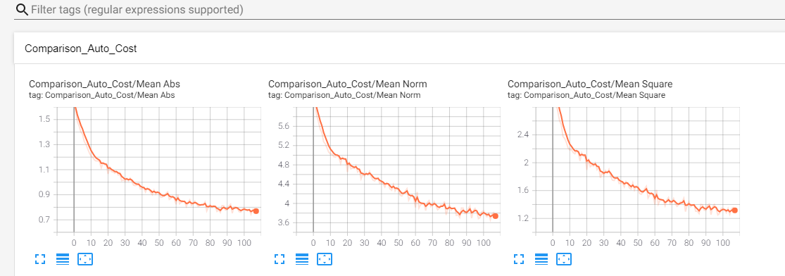
After these values have been calculated we can write them to tensorboard using the tf.summary.scalar() function. We will group them all into a common namespace called Comparison_Auto_Cost.

The last thing we need to talk about: The usage of data[0]. This is because Tensorflow generally assumes a classification task, where data[0] is the train data and data[1] is the train labels. Because we are doing a regression task, we will not use the second part of data. The train_step() method of the parent class also does something similar:

def train_step(self, data):
    """Overwrites the normal train_step. What is different?

    Not much. Even the provided data is expected to be a tuple of (data, classes) (x, y) in classification tasks.
    The data is unpacked and y is discarded, because the Autoencoder Model is a regression task.

    Args:
        data (tuple): The (x, y) data of this train step.

    """
    x, _ = data

from encodermap.misc.distances import periodic_distance

class MyModel(em.models.models.SequentialModel):
    def train_step(self, data):
        parent_class_out = super().train_step(data)

        # call the model on input
        out = self.call(data[0])

        # calculate periodic distance with instance variable self.p containing parameters
        p_dists = periodic_distance(data[0], out, self.p.periodicity)

        # use the different norms
        mean_square = tf.reduce_mean(tf.square(p_dists))
        mean_abs = tf.reduce_mean(tf.abs(p_dists))
        mean_norm = tf.reduce_mean(tf.norm(p_dists, axis=1))

        # write the values to tensorboard
        with tf.name_scope('Comparison_Auto_Cost'):
            tf.summary.scalar('Mean Square', mean_square)
            tf.summary.scalar('Mean Abs', mean_abs)
            tf.summary.scalar('Mean Norm', mean_norm)

        # return the output of the parent's class train_step() function.
        return parent_class_out

my_model = MyModel(dihedrals.shape[1], parameters)

Running EncoderMap with the new model

How do we train the model? We provide an instance of our custom model to EncoderMap’s EncoderMap class and let it handle the rest for us.

Also make sure to execute tensorboard in the correct directory:

$ tensorboard --logdir . --reload_multifile True

If you’re on Google colab, you can use tensorboard, by activating the tensorboard extension:

# %load_ext tensorboard
# %tensorboard --logdir .

e_map = em.EncoderMap(parameters, dihedrals, model=my_model)

Output files are saved to runs/custom_scalars/run0 as defined in 'main_path' in the parameters.
Saved a text-summary of the model and an image in runs/custom_scalars/run0, as specified in 'main_path' in the parameters.

history = e_map.train()

100%|█████████████████████████| 100/100 [00:05<00:00, 19.40it/s, Loss after step 100=31.3]

Saving the model to runs/custom_scalars/run0/saved_model_2024-12-29T13:14:17+01:00.keras. Use `em.EncoderMap.from_checkpoint('runs/custom_scalars/run0')` to load the most recent model, or `em.EncoderMap.from_checkpoint('runs/custom_scalars/run0/saved_model_2024-12-29T13:14:17+01:00.keras')` to load the model with specific weights..
This model has a subclassed encoder, which can be loaded independently. Use `tf.keras.load_model('runs/custom_scalars/run0/saved_model_2024-12-29T13:14:17+01:00_encoder.keras')` to load only this model.
This model has a subclassed decoder, which can be loaded independently. Use `tf.keras.load_model('runs/custom_scalars/run0/saved_model_2024-12-29T13:14:17+01:00_decoder.keras')` to load only this model.

Here’s what Tensorboard should put out: