Logging Custom Images

Welcome

To the third part of EncoderMap’s customization notebooks.

Run this notebook on Google Colab:

Find the documentation of EncoderMap:

https://ag-peter.github.io/encodermap

For Google colab only:

If you’re on Google colab, please uncomment these lines and install EncoderMap.

# !wget https://gist.githubusercontent.com/kevinsawade/deda578a3c6f26640ae905a3557e4ed1/raw/b7403a37710cb881839186da96d4d117e50abf36/install_encodermap_google_colab.sh
# !sudo bash install_encodermap_google_colab.sh

Goals:

In this tuorial you will learn how to add custom images to the “Images” section in TensorBoard. This can be done in two ways:

• Providing ``EncoderMap.add_images_to_tensorboard()` with custom function. <#custom-fn>`__

• Writing a custom Callback, that inherits from ``encodermap.callbacks.EncoderMapBaseCallback`. <#custom-callback>`__

As usual, we will start to import some packages. Along the usual packages we import the built-in package io.

import numpy as np
import encodermap as em
import tensorflow as tf
import plotly.express as px
import plotly.graph_objects as go
from plotly.subplots import make_subplots
import pandas as pd

import io

%matplotlib inline

/home/kevin/git/encoder_map_private/encodermap/__init__.py:194: GPUsAreDisabledWarning: EncoderMap disables the GPU per default because most tensorflow code runs with a higher compatibility when the GPU is disabled. If you want to enable GPUs manually, set the environment variable 'ENCODERMAP_ENABLE_GPU' to 'True' before importing EncoderMap. To do this in python you can run:

import os; os.environ['ENCODERMAP_ENABLE_GPU'] = 'True'

before importing encodermap.
  _warnings.warn(

We will use io to write a png-file to a buffer (not to disk) and provide that puffer to Tensorboard for visualization. But first, let us think about what to plot.

Logging via a custom function

What shall we use as an example in this section? Let’s take the images, that EncoderMap automatically logs during training. These images are generated from a subset of the training data. This subset is passed through the encoder part of the network. The histogram is created from the point in the _gen_hist_matplotlib() function in the encoderamp.misc.summaries.py module.

from encodermap.misc.summaries import _gen_hist_matplotlib
import inspect
print(inspect.getsource(_gen_hist_matplotlib))

def _gen_hist_matplotlib(
    data: np.ndarray,
    hist_kws: dict[str, Any],
) -> tf.Tensor:
    """Creates matplotlib histogram and returns tensorflow Tensor that represents an image.

    Args:
        data (Union[np.ndarray, tf.Tensor]): The xy data to be used. data.ndim should be 2.
            1st dimension the datapoints, 2nd dimension x, y.
        hist_kws (dict): Additional keywords to be passed to matplotlib.pyplot.hist2d().

    Returns:
        tf.Tensor: A tensorflow tensor that can be written to Tensorboard with tf.summary.image().

    """
    plt.close("all")
    matplotlib.use("Agg")  # overwrites current backend of notebook
    plt.figure()
    plt.hist2d(*data.T, **hist_kws)
    buf = io.BytesIO()
    plt.savefig(buf, format="png")
    buf.seek(0)
    image = tf.image.decode_png(buf.getvalue(), 4)
    image = tf.expand_dims(image, 0)
    return image

We can see, that the function that creates the histogram is rather simple. It takes a NumPy array (data: np.ndarray) and keyword arguments (hist_kws: dict[str, Any]) for matplotlib’s plt.hist2d(). But what if we want to use the (x, y) data to plot the a free energy-representation of the 2D latent space. Let’s develop such a function. We will use SKLearn’s make_blobs() function to create the test data.

from sklearn.datasets import make_blobs
data, categories = make_blobs(n_samples=10_000, n_features=2)
px.scatter(x=data[:, 0], y=data[:, 1])

Next, we will create a function called to_free_energy to get the negative log density of a binning of this (x, y) space.

def to_free_energy(data, bins=100):
    """Adapted from PyEMMA.

    Args:
        data (np.ndarray): The low-dimensional data
            as a NumPy array.
        bins (int): The number of bins.

    Returns:
        tuple[np.ndarray, np.ndarray, np.ndarray]:
            A tuple with the x-centers, the y-centers
            as 1D arrays, and the free energy per bin
            as a 2D array.

    """
    # create a histogram
    H, xedges, yedges = np.histogram2d(*data.T, bins=bins)

    # get the bin centers
    x = 0.5 * (xedges[:-1] + xedges[1:])
    y = 0.5 * (yedges[:-1] + yedges[1:])

    # to density
    density = H / float(H.sum())

    # to free energy
    F = np.inf * np.ones_like(H)
    nonzero = density.nonzero()
    F[nonzero] = -np.log(density[nonzero])

    # shift, so that no zeros are in the data
    F[nonzero] -= np.min(F[nonzero])

    # return
    return x, y, F

Let’s test our function:

xx, yy, z = to_free_energy(data)
fig = px.imshow(z.T, origin="lower", width=500, height=500)
fig.show()

Provide this function to EncoderMap

We need to make some adjustments to be able to see similar images in tensorboard.

1. Everything needs to be contained in a single function, that takes the low-dimensional output of the encoder as input.

2. The function needs to return a tensorflow image.

Some other lines we have to add:

• buf = io.BytesIO(). Raw bytecode buffer. These are the actual bytes that would have ended up on your disk, if you would have written the png to it.

def free_energy_tensorboard(lowd):
    # calculate free energy
    H, xedges, yedges = np.histogram2d(*lowd.T, bins=50)
    x = 0.5 * (xedges[:-1] + xedges[1:])
    y = 0.5 * (yedges[:-1] + yedges[1:])

    # to density
    density = H / float(H.sum())

    # to free energy
    F = np.inf * np.ones(shape=H.shape)
    nonzero = density.nonzero()
    F[nonzero] = - np.log(density[nonzero])
    # shift so no zeros happen
    F[nonzero] -= np.min(F[nonzero])

    # actual plotting
    fig = px.imshow(F.T, origin="lower", width=500, height=500)

    # BytesIO
    buf = io.BytesIO()
    fig.write_image(buf)
    buf.seek(0)

    # tensorflow
    image = tf.image.decode_png(buf.getvalue(), 4) # 4 is due to RGBA colors.
    image = tf.expand_dims(image, 0)
    return image

This function will return a tf.Tensor, that we can now log in tensorboard.

free_energy_tensorboard(data)

<tf.Tensor: shape=(1, 500, 500, 4), dtype=uint8, numpy=
array([[[[255, 255, 255, 255],
         [255, 255, 255, 255],
         [255, 255, 255, 255],
         ...,
         [255, 255, 255, 255],
         [255, 255, 255, 255],
         [255, 255, 255, 255]],

        [[255, 255, 255, 255],
         [255, 255, 255, 255],
         [255, 255, 255, 255],
         ...,
         [255, 255, 255, 255],
         [255, 255, 255, 255],
         [255, 255, 255, 255]],

        [[255, 255, 255, 255],
         [255, 255, 255, 255],
         [255, 255, 255, 255],
         ...,
         [255, 255, 255, 255],
         [255, 255, 255, 255],
         [255, 255, 255, 255]],

        ...,

        [[255, 255, 255, 255],
         [255, 255, 255, 255],
         [255, 255, 255, 255],
         ...,
         [255, 255, 255, 255],
         [255, 255, 255, 255],
         [255, 255, 255, 255]],

        [[255, 255, 255, 255],
         [255, 255, 255, 255],
         [255, 255, 255, 255],
         ...,
         [255, 255, 255, 255],
         [255, 255, 255, 255],
         [255, 255, 255, 255]],

        [[255, 255, 255, 255],
         [255, 255, 255, 255],
         [255, 255, 255, 255],
         ...,
         [255, 255, 255, 255],
         [255, 255, 255, 255],
         [255, 255, 255, 255]]]], dtype=uint8)>

Train EncoderMap with our new function.

First get the input data

df = pd.read_csv('asp7.csv')
dihedrals = df.iloc[:,:-1].values.astype(np.float32)
cluster_ids = df.iloc[:,-1].values
print(dihedrals.shape, cluster_ids.shape)
print(df.shape)

(10001, 12) (10001,)
(10001, 13)

Cerate the parameters.

parameters = em.Parameters(
tensorboard=True,
periodicity=2*np.pi,
n_steps=100,
main_path=em.misc.run_path('runs/custom_images')
)

When calling the method add_images_to_tensorboard() we can provide a list of additional functions. That way we can add as much custom functions as we like. In this case, we only add the new free_energy_tensorboard function.

e_map = em.EncoderMap(parameters, dihedrals)
e_map.add_images_to_tensorboard(dihedrals, image_step=1, additional_fns=[free_energy_tensorboard])

Output files are saved to runs/custom_images/run0 as defined in 'main_path' in the parameters.
Saved a text-summary of the model and an image in runs/custom_images/run0, as specified in 'main_path' in the parameters.
Logging images with (10001, 12)-shaped data every 1 epochs to Tensorboard at runs/custom_images/run0

history = e_map.train()

100%|█████████████████████████| 100/100 [00:25<00:00,  3.91it/s, Loss after step 100=32.5]

Saving the model to runs/custom_images/run0/saved_model_2024-12-29T13:55:45+01:00.keras. Use `em.EncoderMap.from_checkpoint('runs/custom_images/run0')` to load the most recent model, or `em.EncoderMap.from_checkpoint('runs/custom_images/run0/saved_model_2024-12-29T13:55:45+01:00.keras')` to load the model with specific weights..
This model has a subclassed encoder, which can be loaded independently. Use `tf.keras.load_model('runs/custom_images/run0/saved_model_2024-12-29T13:55:45+01:00_encoder.keras')` to load only this model.
This model has a subclassed decoder, which can be loaded independently. Use `tf.keras.load_model('runs/custom_images/run0/saved_model_2024-12-29T13:55:45+01:00_decoder.keras')` to load only this model.

Output

Start tensorboard locally via:

$ tensorboard --logdir . --reload_multifile True

If you’re on Google colab, you can use tensorboard by loading the tensorboard extension:

# %load_ext tensorboard
# %tensorboard --logdir .

Here’s what Tensorboard should display:

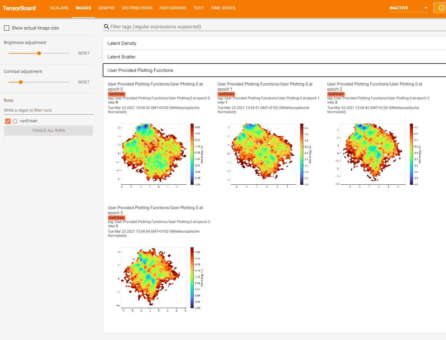
After training we can use the to_free_energy() to plot the latent space after the training is finished.

px.imshow(to_free_energy(e_map.encode())[-1].T, origin="lower", width=500, height=500)

Writing custom callbacks

Writing custom callbacks gives us much more freedom. We can use all kinds of data, that can be provided at the instantiation of a callback. We can also write the images to drive, and so on. We will subclass encodermap.callbacks.EncoderMapBaseCallback and implement our own custom functionality in the on_summary_step() method. Firt, let’s bring up the documentation of that class to see how we can implment our subclass.

?em.callbacks.EncoderMapBaseCallback

Polar coordinates

Then, let’s come up with something to plot to tensorboard. I’ve always like polar plots. So we will analyze the output of the EncoderMap model by polar histograms. Our train data allows that, because we are training on the dihedral (torsion) angles of Asp7. So, the output will always be in a certain range. Let’s get some data and create our plot without the callback first.

output = e_map.decode(e_map.encode())
print(output.min())
print(output.max())

-3.1413832
3.1413581

We can see, that the output lies within the \((-\pi, \pi)\) periodic space.

fig = make_subplots(
    cols=2,
    rows=1,
    specs=[[{"type": "polar"}, {"type": "polar"}]],
    subplot_titles=["input", "output"],
)

# input
radii, bins = np.histogram(dihedrals, bins=25)
bins_degree = np.rad2deg(bins)
widths = np.diff(bins)
fig.add_trace(
    go.Barpolar(
        r=radii,
        theta=bins_degree,
    ),
    col=1,
    row=1,
)

# output
radii, bins = np.histogram(output, bins=25)
bins_degree = np.rad2deg(bins)
widths = np.diff(bins)
fig.add_trace(
    go.Barpolar(
        r=radii,
        theta=bins_degree,
    ),
    col=2,
    row=1,
)
fig.update_layout(
    {
        "height": 500,
        "width": 1000,
    },
)
fig.show()

We also can see that this instance of EncoderMap has some success in recreating the distribution of dihedral angles.

Subclassing EncoderMapBaseCallback

We now know, what we want to plot. We just need to implement it.

class PolarCoordinatesCallback(em.callbacks.EncoderMapBaseCallback):
    # we use our input data as a class attribute
    # (rather than an instance attribute)
    # that way, we can also plot the input diagram
    highd_data = dihedrals.copy()

    def on_summary_step(self, step, logs=None):
        # get output data
        output = self.model(self.highd_data)

        fig = make_subplots(
            cols=2,
            rows=1,
            specs=[[{"type": "polar"}, {"type": "polar"}]],
            subplot_titles=["input", "output"],
        )

        # input
        radii, bins = np.histogram(self.highd_data, bins=25)
        bins_degree = np.rad2deg(bins)
        widths = np.diff(bins)
        fig.add_trace(
            go.Barpolar(
                r=radii,
                theta=bins_degree,
            ),
            col=1,
            row=1,
        )

        # output
        radii, bins = np.histogram(output, bins=25)
        bins_degree = np.rad2deg(bins)
        widths = np.diff(bins)
        fig.add_trace(
            go.Barpolar(
                r=radii,
                theta=bins_degree,
            ),
            col=2,
            row=1,
        )
        fig.update_layout(
            {
                "height": 500,
                "width": 1000,
            },
        )

        # BytesIO
        buf = io.BytesIO()
        fig.write_image(buf)
        buf.seek(0)

        # tensorflow
        image = tf.image.decode_png(buf.getvalue(), 4) # 4 is due to RGBA colors.
        image = tf.expand_dims(image, 0)
        with tf.name_scope("User Provided Plotting Functions"):
            tf.summary.image(f"Polar Plot", image, step=self.steps_counter)

Adding the callback to EncoderMap

Before starting the training we will simply append use the add_callback() method of the EncoderMap instance.

parameters = em.Parameters(
tensorboard=True,
n_steps=100,
periodicity=2*np.pi,
main_path=em.misc.run_path('runs/custom_images')
)

e_map = em.EncoderMap(parameters, dihedrals)
e_map.add_images_to_tensorboard(dihedrals, image_step=1, additional_fns=[free_energy_tensorboard])

# add the new callback
e_map.add_callback(PolarCoordinatesCallback)

Output files are saved to runs/custom_images/run1 as defined in 'main_path' in the parameters.
Saved a text-summary of the model and an image in runs/custom_images/run1, as specified in 'main_path' in the parameters.
Logging images with (10001, 12)-shaped data every 1 epochs to Tensorboard at runs/custom_images/run1

history = e_map.train()

100%|█████████████████████████| 100/100 [00:26<00:00,  3.82it/s, Loss after step 100=29.6]

Saving the model to runs/custom_images/run1/saved_model_2024-12-29T13:56:12+01:00.keras. Use `em.EncoderMap.from_checkpoint('runs/custom_images/run1')` to load the most recent model, or `em.EncoderMap.from_checkpoint('runs/custom_images/run1/saved_model_2024-12-29T13:56:12+01:00.keras')` to load the model with specific weights..
This model has a subclassed encoder, which can be loaded independently. Use `tf.keras.load_model('runs/custom_images/run1/saved_model_2024-12-29T13:56:12+01:00_encoder.keras')` to load only this model.
This model has a subclassed decoder, which can be loaded independently. Use `tf.keras.load_model('runs/custom_images/run1/saved_model_2024-12-29T13:56:12+01:00_decoder.keras')` to load only this model.

Output

The output from Tensorboard could look something like this:

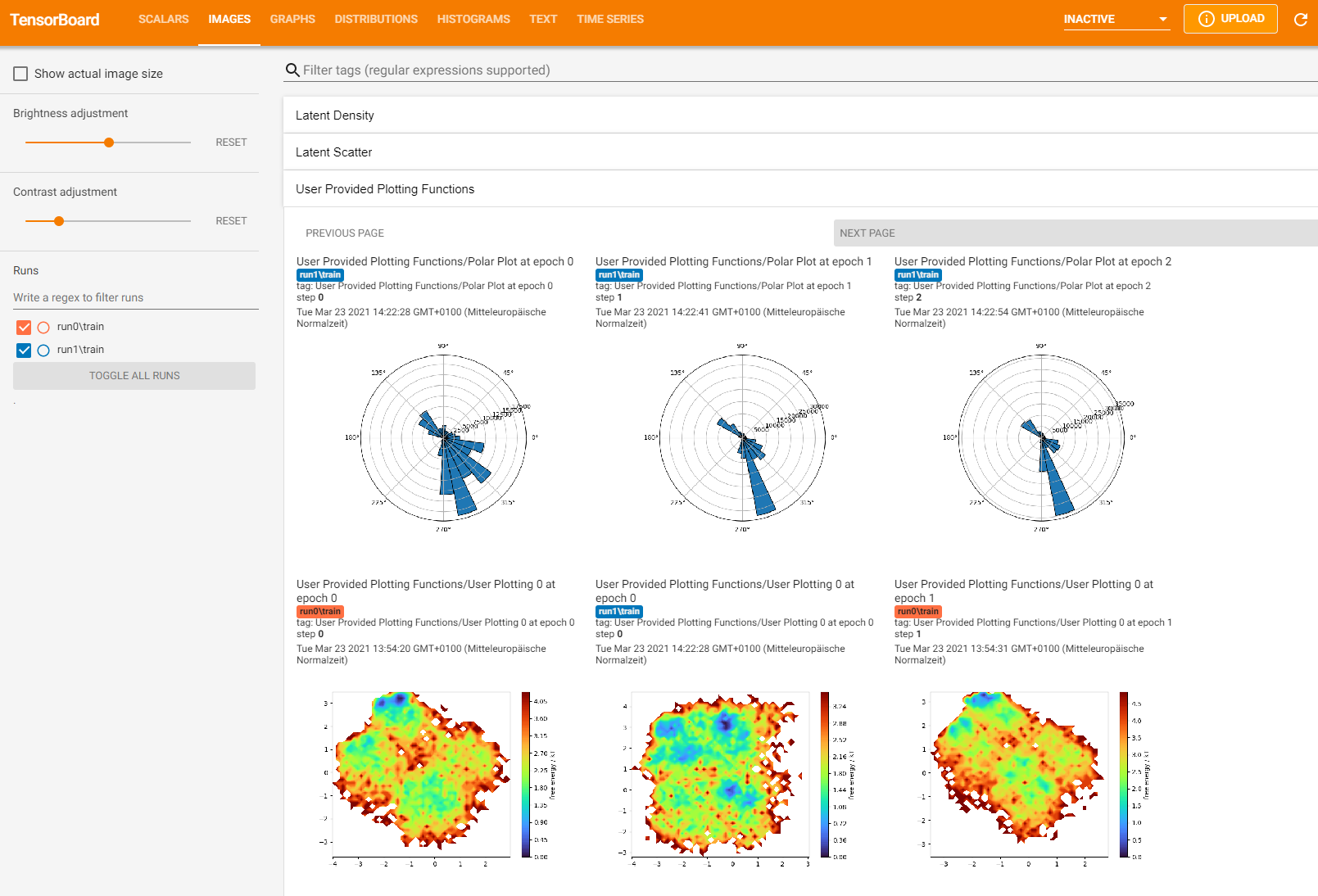
We can clearly see our polar histogram function. Furthermore, we can see, that at training step 10 the EncoderMap network was not yet able to reproduce the input dihedral distribution.

Conclusion

Using the tools provided in this notebook, you will be able to customize EncoderMap to your liking. Using images to visualize the output of the neural network is a much better visual aid, than just looking at graphs of raw data.