Advanced Usage: Asp 7

Run this notebook on Google Colab:

Find the documentation of EncoderMap:

https://ag-peter.github.io/encodermap

Goals:

In this tutorial you will learn:

• What’s different when data lies in a periodic space.

• How to visualize and observe training progression using ``Tensorboard`. <#tensorboard>`__

• How to use EncoderMap’s InteractivePlotting session.

For Google colab only:

If you’re on Google colab, please uncomment these lines and install EncoderMap.

# !wget https://gist.githubusercontent.com/kevinsawade/deda578a3c6f26640ae905a3557e4ed1/raw/b7403a37710cb881839186da96d4d117e50abf36/install_encodermap_google_colab.sh
# !sudo bash install_encodermap_google_colab.sh

If you’re on Google colab, you also want to download the data we will use in this notebook.

# !wget https://raw.githubusercontent.com/AG-Peter/encodermap/main/tutorials/notebooks_starter/asp7.csv
# !wget https://raw.githubusercontent.com/AG-Peter/encodermap/main/tutorials/notebooks_starter/asp7.pdb
# !wget https://raw.githubusercontent.com/AG-Peter/encodermap/main/tutorials/notebooks_starter/asp7.xtc

Primer

Imports and load data

In this tutorial we will use example data from a molecular dynamics simulation and learn more about advanced usage of EncoderMap. Encoder map can create low-dimensional maps of the vast conformational spaces of molecules. This allows easy identification of the most common molecular conformations and helps to understand the relations between these conformations. In this example, we will use data from a simulation of a simple peptide: hepta-aspartic-acid.

First we need to import some libraries:

import encodermap as em
import numpy as np
import plotly.express as px
import plotly.io as pio
from math import pi
try:
    from google.colab import data_table, output
    data_table.enable_dataframe_formatter()
    output.enable_custom_widget_manager()
    renderer = "colab"
except ModuleNotFoundError:
    renderer = "plotly_mimetype+notebook"
pio.renderers.default = renderer

/home/kevin/git/encoder_map_private/encodermap/__init__.py:194: GPUsAreDisabledWarning: EncoderMap disables the GPU per default because most tensorflow code runs with a higher compatibility when the GPU is disabled. If you want to enable GPUs manually, set the environment variable 'ENCODERMAP_ENABLE_GPU' to 'True' before importing EncoderMap. To do this in python you can run:

import os; os.environ['ENCODERMAP_ENABLE_GPU'] = 'True'

before importing encodermap.
  _warnings.warn(

Next, we need to load the input data. Different kinds of variables can be used to describe molecular conformations: e.g. Cartesian coordinates, distances, angles, dihedrals… In principle EncoderMap can deal with any of these inputs, however, some are better suited than others. The molecular conformation does not change when the molecule is translated or rotated. The chosen input variables should reflect that and be translationally and rotationally invariant.

In this example we use the backbone dihedral angles phi and psi as input as they are translationally and rotationally invariant and describe the backbone of a protein/peptide very well.

The “asp7.csv” file contains one column for each dihedral and one row for each frame of the trajectory. Additionally, the last column contains a cluster_id from a gromos clustering which we can later use for comparison. We can load this data using np.loadtxt():

csv_path = "asp7.csv"
data = np.loadtxt(csv_path, skiprows=1, delimiter=",")
dihedrals = data[:, :-1]
cluster_ids = data[:, -1]

We can view the molecular dynamics simulation right here in this jupyter notebook using the nglview package. This cell loads the asp7.xtc trajectory and asp7.pdb topology file and displays them as a ball and stick representation.

If you don’t have access to these files, you can replace the line

traj = md.load('asp7.xtc', top='asp7.pdb')

with

traj = md.load_pdb('https://files.rcsb.org/view/1YUF.pdb')

to load a small molecular conformation ensemble from the protein database.

Hint:

Sometimes the view can be not centered. Use the ‘center’ button in the gui to center the structure.

import plotly.io as pio
pio.templates.default = "plotly_white"
traj = em.load('asp7.pdb')
em.plot.plot_ball_and_stick(traj, highlight="dihedrals")

/home/kevin/git/encoder_map_private/encodermap/loading/features.py:1005: UserWarning:

You requested a `em.loading.features.Feature` to calculate features in a periodic box, using the minimum image convention, but the trajectory you provided does not have unitcell information. If this feature will later be supplied with trajectories with unitcell information, an Exception will be raised, to make sure distances/angles are calculated correctly.

import nglview as nv
import mdtraj as md
traj = md.load('asp7.xtc', top='asp7.pdb')
traj.center_coordinates()
view = nv.show_mdtraj(traj, gui=True)
view.clear_representations()
view.add_representation('ball+stick')
view

Periodic variables

Periodic variables pose a problem, when we implement a distance metric between two values in a periodic space. When the input space is not-periodic, the euclidean distacen between two points (\(p\) and \(q\)) is given as:

\begin{equation} d(p, q) = \sqrt{\left( p-q \right)^2} \end{equation}

This equation does not apply when p and q are in a periodic space. Take angle values as an example. Let us assume \(p\) and \(q\) lie in a periodic space of \((-180^\circ, 180^\circ]\) (\(-180^\circ\) is not included, \(180^\circ\) is included) and have the values \(p=-100^\circ\) and \(q=150^\circ\). Plugging that into formula, we get:

\begin{align} d(p, q) &= \sqrt{\left( -100-150 \right)^2}\\ &= \sqrt{\left( -250 \right)^2}\\ &=250 \end{align}

However, the distance between these two points is not \(250^\circ\), but \(110^\circ\).

import plotly.graph_objects as go
one = go.Scatterpolar(
    r=np.full((100, ), 1),
    theta=np.linspace(-100, 150, 100),
    name="250 deg distance",
    hovertemplate="250 deg distance",
)
two = go.Scatterpolar(
    r=np.full((100, ), 1),
    theta=np.linspace(0, 110, 100) - 210,
    hovertemplate="110 deg distance",
)
fig = go.Figure(
    data=[one, two],
    layout={
        "polar": {
            "radialaxis": {
                "showticklabels": False,
                "showgrid": False,
                "range": [0.5, 1.5],
            },
            "angularaxis": {
                "tickmode": "array",
                "tickvals": [0, 45, 90, 135, 180, 225, 270, 315],
                "ticktext": [0, 45, 90, 135, 180, -135, -90, -45],
            },
        },
        "showlegend": False,
    },
)
fig.show()

The distance in periodic spaces can be corrected using this formula:

\begin{equation} d_{360}(p, q) = min\left( d(p, q), 360 - d(p, q) \right) \end{equation}

Furthermore, during training the the angle values \(\theta\) are converted into value pairs \(\left( sin(\theta), cos(\theta) \right)\) to represent this.

Parameter selection

Similarly to the previous example, we need to set some parameters. In contrast to the Cube example we now have periodic input data. The dihedral angles are in radians with a 2pi periodicity. We also set some further parameters but don’t bother for now.

parameters = em.Parameters()
parameters.main_path = em.misc.run_path("runs/asp7")
parameters.n_steps = 100
parameters.dist_sig_parameters = (4.5, 12, 6, 1, 2, 6)
parameters.periodicity = 2*pi
parameters.l2_reg_constant = 10.0
parameters.summary_step = 1
parameters.tensorboard = True

em.plot.distance_histogram_interactive(
    dihedrals[::10],
    parameters.periodicity,
    initial_guess=parameters.dist_sig_parameters,
    bins=50,
)

Next, we can run the dimensionality reduction:

e_map = em.EncoderMap(parameters, dihedrals)

Output files are saved to runs/asp7/run0 as defined in 'main_path' in the parameters.
Saved a text-summary of the model and an image in runs/asp7/run0, as specified in 'main_path' in the parameters.

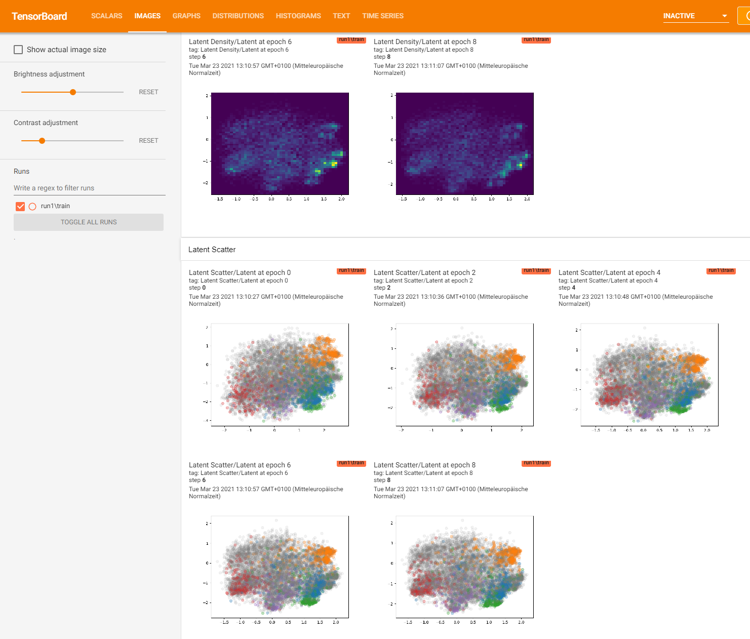
The new tensorflow 2 version of EncoderMap allows you to also view the output of the latent space during the training. Switch that feature on with e_map.add_images_to_tensorboard().

e_map.add_images_to_tensorboard()

Logging images with (10000, 12)-shaped data every 1 epochs to Tensorboard at runs/asp7/run0

history = e_map.train()

100%|██████████████████████| 100/100 [00:19<00:00,  5.11it/s, Loss after step 100=1.92e+3]

Saving the model to runs/asp7/run0/saved_model_2024-12-29T13:06:42+01:00.keras. Use `em.EncoderMap.from_checkpoint('runs/asp7/run0')` to load the most recent model, or `em.EncoderMap.from_checkpoint('runs/asp7/run0/saved_model_2024-12-29T13:06:42+01:00.keras')` to load the model with specific weights..
This model has a subclassed encoder, which can be loaded independently. Use `tf.keras.load_model('runs/asp7/run0/saved_model_2024-12-29T13:06:42+01:00_encoder.keras')` to load only this model.
This model has a subclassed decoder, which can be loaded independently. Use `tf.keras.load_model('runs/asp7/run0/saved_model_2024-12-29T13:06:42+01:00_decoder.keras')` to load only this model.

project all dihedrals to the low-dimensional space…

low_d_projection = e_map.encode(dihedrals)

and plot the result:

import pandas as pd

# define max clusters
max_clusters = 5

# remove unwanted clusters
colors = cluster_ids.copy()
colors[colors > max_clusters] = 0
colors = colors.astype(int).astype(str)

# plot
px.scatter(
    data_frame=pd.DataFrame(
        {
            "x": low_d_projection[:, 0],
            "y": low_d_projection[:, 1],
            "color": colors,
        }
    ),
    x="x",
    y="y",
    color="color",
    opacity=0.5,
    color_discrete_map={
        "0": "rgba(100, 100, 100, 0.2)",
    },
    labels={
        "x": "x in a.u.",
        "y": "y in a.u.",
        "color": "cluster",
    },
    width=500,
    height=500,
)

In the above map points from different clusters (different colors) should be well separated. However, if you didn’t change the parameters, they are probably not. Some of our parameter settings appear to be unsuitable. Let’s see how we can find out what goes wrong.

The history element returned by e_map.train() is an instance of tf.keras.callbacks.History, which contains the loss during the training steps:

loss = np.asarray(history.history["loss"])

px.line(
    x=np.arange(len(loss)),
    y=loss,
    labels={
        "x": "training step",
        "y": "loss",
    },
    width=500,
    height=500,
)

Visualize Learning with TensorBoard

Running tensorboard on Google colab

To use tensorboard in google colabs notebooks, you neet to first load the tensorboard extension

%load_ext tensorboard

And then activate it with:

%tensorboard --logdir .

The next code cell contains these commands. Uncomment them and then continue.

Running tensorboard locally

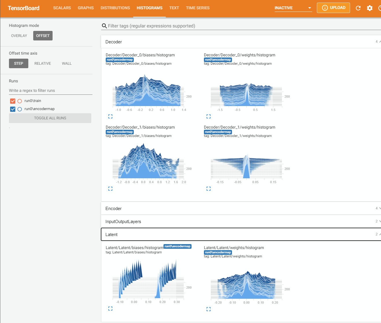
TensorBoard is a visualization tool from the machine learning library TensorFlow which is used by the EncoderMap package. During the dimensionality reduction step, when the neural network autoencoder is trained, several readings are saved in a TensorBoard format. All output files are saved to the path defined in parameters.main_path. Navigate to this location in a shell and start TensorBoard. Change the paramter Tensorboard to True to make Encodermap log to Tensorboard.

In case you run this tutorial in the provided Docker container you can open a new console inside the container by typing the following command in a new system shell.

docker exec -it emap bash

Navigate to the location where all the runs are saved. e.g.:

cd notebooks_easy/runs/asp7/

Start TensorBoard in this directory with:

tensorboard --logdir .

You should now be able to open TensorBoard in your webbrowser on port 6006.

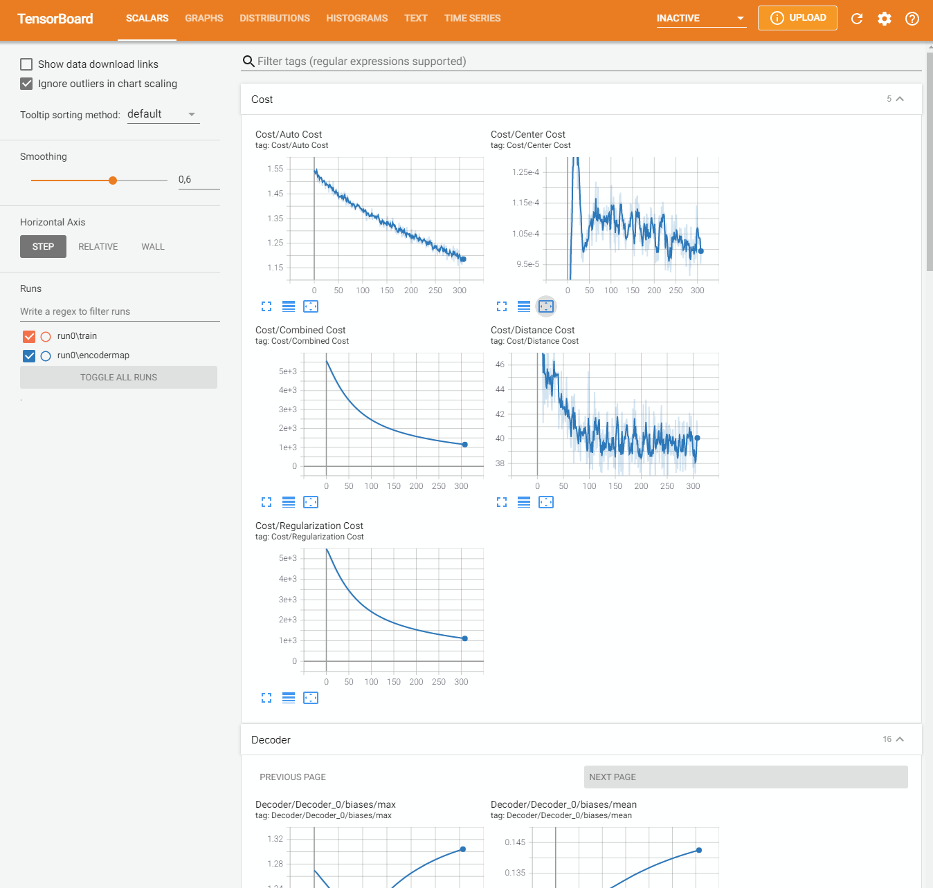
0.0.0.0:6006 or 127.0.0.1:6006

In the SCALARS tab of TensorBoard you should see among other values the overall cost and different contributions to the cost. The two most important contributions are auto_cost and distance_cost. auto_cost indicates differences between the inputs and outputs of the autoencoder. distance_cost is the part of the cost function which compares pairwise distances in the input space and the low-dimensional (latent) space.

Fixing Reloading issues Using Tensorboard we often encountered some issues while training multiple models and writing mutliple runs to Tensorboard’s logdir. Reloading the data and event refreshing the web page did not display the data of the current run. We needed to kill tensorboard and restart it in order to see the new data. This issue was fixed by setting reload_multifile True.

tensorboard --logdir . --reload_multifile True

In your case, probably the overall cost as well as the auto_cost and the distance_cost are still decreasing after all training iterations. This tells us that we can simply improve the result by increasing the number of training steps. The following cell contains the same code as above. Set a larger number of straining steps to improve the result (e.g. 3000).

When you’re on Goole Colab, you can load the Tensorboard extension with:

# %load_ext tensorboard
# %tensorboard --logdir .

# Define parameters
parameters = em.Parameters(
    main_path=em.misc.run_path("runs/asp7"),
    n_steps=100,
    dist_sig_parameters=(4.5, 12, 6, 1, 2, 6),
    periodicity=2*pi,
    l2_reg_constant=10,
    summary_step=1,
    tensorboard=True
)

# Instantiate the EncoderMap class
e_map = em.EncoderMap(parameters, dihedrals)


# this function returns rgba() values, that plotly.express.scatter understands
def colors_from_cluster_ids(cluster_ids, max_clusters=10):
    import plotly as plt
    colors = np.full(shape=(len(cluster_ids), ), fill_value="rgba(125, 125, 125, 0.1)")
    # colors = np.full(shape=(len(cluster_ids), 4), fill_value=(.5, .5, .5, .1))
    for i in range(2, max_clusters + 2):
        where = np.where(cluster_ids == i)
        color = plt.colors.DEFAULT_PLOTLY_COLORS[i - 2]
        color = color.replace(")", ", 0.3)").replace("rgb", "rgba")
        colors[where] = color
    return colors

# Logging images to Tensorboard can greatly reduce performance.
# So they need to be specifically turned on
# with the .add_images_to_tensorboard() method
e_map.add_images_to_tensorboard(
    data=dihedrals,
    image_step=2,
    plotly_scatter_kws={
        'size_max': 1,
        'color': colors_from_cluster_ids(cluster_ids, 5),
    },
    backend="plotly",
    save_to_disk=True,
)

history = e_map.train()

Output files are saved to runs/asp7/run1 as defined in 'main_path' in the parameters.
Saved a text-summary of the model and an image in runs/asp7/run1, as specified in 'main_path' in the parameters.
Logging images with (10001, 12)-shaped data every 2 epochs to Tensorboard at runs/asp7/run1

100%|██████████████████████| 100/100 [00:40<00:00,  2.46it/s, Loss after step 100=1.91e+3]

Saving the model to runs/asp7/run1/saved_model_2024-12-29T13:07:23+01:00.keras. Use `em.EncoderMap.from_checkpoint('runs/asp7/run1')` to load the most recent model, or `em.EncoderMap.from_checkpoint('runs/asp7/run1/saved_model_2024-12-29T13:07:23+01:00.keras')` to load the model with specific weights..
This model has a subclassed encoder, which can be loaded independently. Use `tf.keras.load_model('runs/asp7/run1/saved_model_2024-12-29T13:07:23+01:00_encoder.keras')` to load only this model.
This model has a subclassed decoder, which can be loaded independently. Use `tf.keras.load_model('runs/asp7/run1/saved_model_2024-12-29T13:07:23+01:00_decoder.keras')` to load only this model.

The molecule conformations form different clusters (different colors) should be separated a bit better now. In TensorBoard you should see the cost curves for this new run. When the cost curve becomes more or less flat towards the end, longer training does not make sense.

The resulting low-dimensional projection is probably still not very detailed and clusters are probably not well separated. Currently we use a regularization constant parameters.l2_reg_constant = 10.0. The regularization constant influences the complexity of the network and the map. A high regularization constant will result in a smooth map with little details. A small regularization constant will result in a rougher more detailed map.

Go back to the previous cell and decrease the regularization constant (e.g. parameters.l2_reg_constant = 0.001). Play with different settings to improve the separation of the clusters in the map. Have a look at TensorBoard to see how the cost changes for different parameters.

lowd = e_map.encode(dihedrals)

fig = px.scatter(
    x=lowd[:, 0],
    y=lowd[:, 1],
    color=colors_from_cluster_ids(cluster_ids, 5),
    height=500,
    width=500,
    size_max=0.1,
    opacity=0.4,
    labels={
        "x": "x in a.u.",
        "y": "y in a.u.",
    },
)
fig.update_layout(showlegend=False)
fig.show()

Here is what you can see in Tensorboard:

Save and Load

Once you are satisfied with your EncoderMap, you might want to save the result. The good news is: Encoder map automatically saves checkpoints during the training process in parameters.main_path. The frequency of writing checkpoints can be defined with patameters.checkpoint_step. Also, your selected parameters are saved in a file called parameters.json. Navigate to the driectory of your last run and open this parameters.json file in some text editor. You should find all the parameters that we have set so far. You also find some parameters which were not set by us specifically and where EncoderMap used its default values.

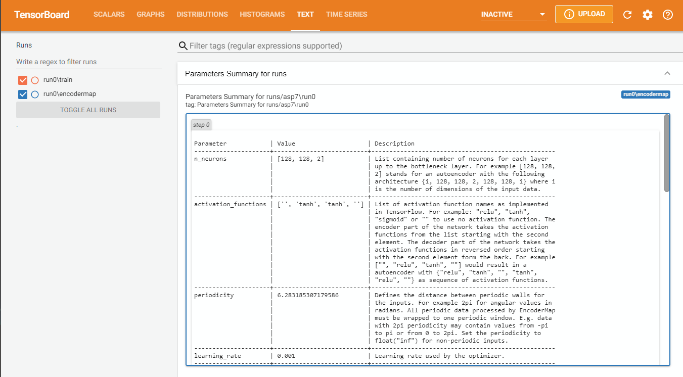
Let’s start by looking at the parameters from the last run and printing them in a nicely formatted table with the .parameters attribute.

loaded_parameters = em.Parameters.from_file('runs/asp7/run0/parameters.json')
print(loaded_parameters.parameters)

Seems like the parameter file was moved to another directory. Parameter file is updated ...
    Parameter                 | Value                    | Description
    --------------------------+--------------------------+---------------------------------------------------
    n_neurons                 | [128, 128, 2]            | List containing number of neurons for each layer
                              |                          | up to the bottleneck layer. For example [128, 128,
                              |                          | 2] stands for an autoencoder with the following
                              |                          | architecture {i, 128, 128, 2, 128, 128, i} where i
                              |                          | is the number of dimensions of the input data.
                              |                          | These are Input/Output Layers that are not
                              |                          | trained.
    --------------------------+--------------------------+---------------------------------------------------
    activation_functions      | ['', 'tanh', 'tanh', ''] | List of activation function names as implemented
                              |                          | in TensorFlow. For example: "relu", "tanh",
                              |                          | "sigmoid" or "" to use no activation function. The
                              |                          | encoder part of the network takes the activation
                              |                          | functions from the list starting with the second
                              |                          | element. The decoder part of the network takes the
                              |                          | activation functions in reversed order starting
                              |                          | with the second element form the back. For example
                              |                          | ["", "relu", "tanh", ""] would result in a
                              |                          | autoencoder with {"relu", "tanh", "", "tanh",
                              |                          | "relu", ""} as sequence of activation functions.
    --------------------------+--------------------------+---------------------------------------------------
    periodicity               | 6.283185307179586        | Defines the distance between periodic walls for
                              |                          | the inputs. For example 2pi for angular values in
                              |                          | radians. All periodic data processed by EncoderMap
                              |                          | must be wrapped to one periodic window. E.g. data
                              |                          | with 2pi periodicity may contain values from -pi
                              |                          | to pi or from 0 to 2pi. Set the periodicity to
                              |                          | float("inf") for non-periodic inputs.
    --------------------------+--------------------------+---------------------------------------------------
    learning_rate             | 0.001                    | Learning rate used by the optimizer.
    --------------------------+--------------------------+---------------------------------------------------
    n_steps                   | 100                      | Number of training steps.
    --------------------------+--------------------------+---------------------------------------------------
    batch_size                | 256                      | Number of training points used in each training
                              |                          | step
    --------------------------+--------------------------+---------------------------------------------------
    summary_step              | 1                        | A summary for TensorBoard is writen every
                              |                          | summary_step steps.
    --------------------------+--------------------------+---------------------------------------------------
    checkpoint_step           | 5000                     | A checkpoint is writen every checkpoint_step
                              |                          | steps.
    --------------------------+--------------------------+---------------------------------------------------
    dist_sig_parameters       | [4.5, 12, 6, 1, 2, 6]    | Parameters for the sigmoid functions applied to
                              |                          | the high- and low-dimensional distances in the
                              |                          | following order (sig_h, a_h, b_h, sig_l, a_l, b_l)
    --------------------------+--------------------------+---------------------------------------------------
    distance_cost_scale       | 500                      | Adjusts how much the distance based metric is
                              |                          | weighted in the cost function.
    --------------------------+--------------------------+---------------------------------------------------
    auto_cost_scale           | 1                        | Adjusts how much the autoencoding cost is weighted
                              |                          | in the cost function.
    --------------------------+--------------------------+---------------------------------------------------
    auto_cost_variant         | mean_abs                 | defines how the auto cost is calculated. Must be
                              |                          | one of: * `mean_square` * `mean_abs` * `mean_norm`
    --------------------------+--------------------------+---------------------------------------------------
    center_cost_scale         | 0.0001                   | Adjusts how much the centering cost is weighted in
                              |                          | the cost function.
    --------------------------+--------------------------+---------------------------------------------------
    l2_reg_constant           | 10.0                     | Adjusts how much the L2 regularisation is weighted
                              |                          | in the cost function.
    --------------------------+--------------------------+---------------------------------------------------
    gpu_memory_fraction       |                          | Specifies the fraction of gpu memory blocked. If
                              |                          | set to 0, memory is allocated as needed.
    --------------------------+--------------------------+---------------------------------------------------
    analysis_path             |                          | A path that can be used to store analysis
    --------------------------+--------------------------+---------------------------------------------------
    id                        |                          | Can be any name for the run. Might be useful for
                              |                          | example for specific analysis for different data
                              |                          | sets.
    --------------------------+--------------------------+---------------------------------------------------
    model_api                 | sequential               | A string defining the API to be used to build the
                              |                          | keras model. Defaults to `sequntial`. Possible
                              |                          | strings are: * `functional` will use keras'
                              |                          | functional API. * `sequential` will define a keras
                              |                          | Model, containing two other models with the
                              |                          | Sequential API. These two models are encoder and
                              |                          | decoder. * `custom` will create a custom Model
                              |                          | where even the layers are custom.
    --------------------------+--------------------------+---------------------------------------------------
    loss                      | emap_cost                | A string defining the loss function. Defaults to
                              |                          | `emap_cost`. Possible losses are: *
                              |                          | `reconstruction_loss` will try to train output ==
                              |                          | input * `mse`: Returns a mean squared error loss.
                              |                          | * `emap_cost` is the EncoderMap loss function.
                              |                          | Depending on the class `Autoencoder`, `Encodermap,
                              |                          | `ADCAutoencoder`, different contributions are used
                              |                          | for a combined loss. Autoencoder uses atuo_cost,
                              |                          | reg_cost, center_cost. EncoderMap class adds
                              |                          | sigmoid_loss.
    --------------------------+--------------------------+---------------------------------------------------
    training                  | auto                     | A string defining what kind of training is
                              |                          | performed when autoencoder.train() is callsed. *
                              |                          | `auto` does a regular model.compile() and
                              |                          | model.fit() procedure. * `custom` uses gradient
                              |                          | tape and calculates losses and gradients manually.
    --------------------------+--------------------------+---------------------------------------------------
    batched                   | True                     | Whether the dataset is batched or not.
    --------------------------+--------------------------+---------------------------------------------------
    tensorboard               | True                     | Whether to print tensorboard information. Defaults
                              |                          | to False.
    --------------------------+--------------------------+---------------------------------------------------
    seed                      |                          | Fixes the state of all operations using random
                              |                          | numbers. Defaults to None.
    --------------------------+--------------------------+---------------------------------------------------
    current_training_step     | 100                      | The current training step. Aids in reloading of
                              |                          | models.
    --------------------------+--------------------------+---------------------------------------------------
    write_summary             | True                     | If True writes a summar.txt of the models into
                              |                          | main_path if `tensorboard` is True, summaries will
                              |                          | also be written.
    --------------------------+--------------------------+---------------------------------------------------
    trainable_dense_to_sparse |                          | When using different topologies to train the
                              |                          | AngleDihedralCartesianEncoderMap, some inputs
                              |                          | might be sparse, which means, they have missing
                              |                          | values. Creating a dense input is done by first
                              |                          | passing these sparse tensors through
                              |                          | `tf.keras.layers.Dense` layers. These layers have
                              |                          | trainable weights, and if this parameter is True,
                              |                          | these weights will be changed by the optimizer.
    --------------------------+--------------------------+---------------------------------------------------
    using_hypercube           |                          | This parameter is not meant to be set by the user.

Before we can reload our trained network we need to save it manually, because the checkpoint step was set to 5000 and we did only write a checkpoint at 0 (random initial weights). We call e_map.save() to do so.

e_map.save()

Saving the model to runs/asp7/run1/saved_model_2024-12-29T13:07:23+01:00.keras. Use `em.EncoderMap.from_checkpoint('runs/asp7/run1')` to load the most recent model, or `em.EncoderMap.from_checkpoint('runs/asp7/run1/saved_model_2024-12-29T13:07:23+01:00.keras')` to load the model with specific weights..
This model has a subclassed encoder, which can be loaded independently. Use `tf.keras.load_model('runs/asp7/run1/saved_model_2024-12-29T13:07:23+01:00_encoder.keras')` to load only this model.
This model has a subclassed decoder, which can be loaded independently. Use `tf.keras.load_model('runs/asp7/run1/saved_model_2024-12-29T13:07:23+01:00_decoder.keras')` to load only this model.

PosixPath('runs/asp7/run1')

And now we reload it.

# get the most recent run directory
from pathlib import Path
import re

latest_run_dir = Path("runs/asp7").glob("run*")
latest_run_dir = sorted(latest_run_dir, key=lambda x: int(re.findall(r"\d+", str(x))[0]))[0]
loaded_e_map = em.EncoderMap.from_checkpoint(latest_run_dir)

Seems like the parameter file was moved to another directory. Parameter file is updated ...
Output files are saved to runs/asp7/run0 as defined in 'main_path' in the parameters.
Saved a text-summary of the model and an image in runs/asp7/run0, as specified in 'main_path' in the parameters.

Now we are finished with loading and we can for example use the loaded EncoderMap object to project data to the low_dimensional space and plot the result:

import pandas as pd

# define max clusters
max_clusters = 5

# remove unwanted clusters
colors = cluster_ids.copy()
colors[colors > max_clusters] = 0
colors = colors.astype(int).astype(str)

# plot
px.scatter(
    data_frame=pd.DataFrame(
        {
            "x": lowd[:, 0],
            "y": lowd[:, 1],
            "color": colors,
        }
    ),
    x="x",
    y="y",
    color="color",
    opacity=0.5,
    color_discrete_map={
        "0": "rgba(100, 100, 100, 0.2)",
    },
    labels={
        "x": "x in a.u.",
        "y": "y in a.u.",
        "color": "cluster",
    },
    width=500,
    height=500,
)

Generate Molecular Conformations

Already in the cube example, you have seen that with EncoderMap it is not only possible to project points to the low-dimensional space. Also, a projection of low-dimensional points into the high-dimensional space is possible.

Here, we will use a tool form the EncoderMap library to interactively select a path in the low-dimensional map called. We will project points along this path into the high-dimensional dihedral space, and use these dihedrals to reconstruct molecular conformations. This can be very useful to explore the landscape an to see what changes occur in the molecular conformation going from one cluster to another.

The next cell instantiates the InteractivePlotting class of EncoderMap. Inside the main plotting area, you can click on points and their corresponding molecular conformation is displayed in the right window. The Trace plot contains the high-dimensional data (in this case the dihedrals) that this point was projected from. Picking up the Lasso tool from the toolbar, you can draw a lasso selection around some points. Pressing Cluster afterwards will display 10 structures from all of the structures you selected. You can adjust this number with the Size slider.

More interesting is the Path tool which can be used, when the density is displayed. With this tool you can generate molecular conformations from a path in the latent space. You don’t need to pick up a tool from the toolbar to draw a path. Just switch to density with the Density button. After you have drawn your path, click Generate to generate the molecular conformations from the low-dimensional points that you just drew.

In either case, hitting Save will sasve your cluster or path into the training directory of the EncoderMap class (where alsi Tensorboard stuff is put).

Give the InteractivePlotting a try. We would like to hear your feedback at GitHub.

sess = em.InteractivePlotting(
    e_map,
    trajs="asp7.xtc",
    lowd_data=lowd,
    highd_data=dihedrals,
    top='asp7.pdb',
    ball_and_stick=True,
)

As backbone dihedrals contain no information about the side-chains, only the backbone of the molecule can be reconstructed. In case the generated conformations change very abruptly it might be sensible to increase the regularization constant to obtain a smoother representation. If the generated conformations along a path are not changing at all, the regularization is probably to strong and prevents the network form generating different conformations.

Conclusion

In this tutorial we applied EncoderMap to a molecular system. You have learned how to monitor the EncoderMap training procedure with TensorBoard, how to restore previously saved EncoderMaps and how to generate Molecular conformations using the InteractivePlotting session.