Customize EncoderMap: Custom loss functions

Welcome

Welcome to the second part of the customization section.

Run this notebook on Google Colab:

Find the documentation of EncoderMap:

https://ag-peter.github.io/encodermap

Goals:

In this tuorial you will learn:

• A few general concepts about loss functions.

• What loss functions are implemented in EncoderMap.

• How you can write your own loss functions.

• Another example for a custom loss function.

For Google colab only

If you’re on Google colab, please uncomment these lines and install EncoderMap.

# !wget https://gist.githubusercontent.com/kevinsawade/deda578a3c6f26640ae905a3557e4ed1/raw/b7403a37710cb881839186da96d4d117e50abf36/install_encodermap_google_colab.sh
# !sudo bash install_encodermap_google_colab.sh

Import Libraries

In this tutorial we will learn how to write our own loss functions and add them to EncoderMap. Let us start with the imports:

import numpy as np
import pandas as pd
import plotly
import plotly.express as px
import plotly.graph_objects as go
import plotly.subplots as ps
import tensorflow as tf

import encodermap as em

from pathlib import Path

%load_ext autoreload
%autoreload 2

/home/kevin/git/encoder_map_private/encodermap/__init__.py:194: GPUsAreDisabledWarning: EncoderMap disables the GPU per default because most tensorflow code runs with a higher compatibility when the GPU is disabled. If you want to enable GPUs manually, set the environment variable 'ENCODERMAP_ENABLE_GPU' to 'True' before importing EncoderMap. To do this in python you can run:

import os; os.environ['ENCODERMAP_ENABLE_GPU'] = 'True'

before importing encodermap.
  _warnings.warn(

What are loss functions

Loss functions in EncoderMap are small pieces of code, that take some inputs and return scalar values. We can easily come up with a loss function ourselves, when we think about a linear regression. First let us create some example data in a \(\mathbb{R}^2\) space. Each point \(i\) is defined by an x-value \(x^{(i)}\) and a true y-value \(y^{(i)}\).

x = np.linspace(0, 10, 200)
y = np.linspace(0, 10, 200)

# add noise
y += (np.random.random((200, )) - 0.5) * (np.abs(y - 5) + 1)

fig = px.scatter(x=x, y=y, labels={"x": "x", "y": "y"})
fig.show()

The model describing our data will be a linear function without a y-intercept. This model takes in an actual x-value of the data \(x\), multiplies it with a value \(w\) and produces a prediction \(\hat{y}\).

\begin{equation} \hat{y} = wx \end{equation}

And the cost function \(J(w)\) is defined as the squared distance between a sample \(y\) and our prediction \(\hat{y}\). Our cost function is a function of the parameter \(w\):

\begin{align} J(w) &= \frac{1}{2m} \sum_{i=1}^m \left( \hat{y}^{(i)} - y^{(i)} \right) ^ 2\\ &= \frac{1}{2m} \sum_{i=1}^m \left( wx^{(i)} - y^{(i)} \right) ^ 2 \end{align}

We can plot this loss function using a range of \(w\) values:

def y_hat(x, w):
    return w * x

def J(w):
    loss = 0
    for x_sample, y_true in zip(x, y):
        y_pred = y_hat(x_sample, w)
        loss += (y_pred - y_true) ** 2
    loss /= (2 * len(x))
    return loss

test_w = np.linspace(0, 2, 20)
test_J = [J(w) for w in test_w]

fig = px.line(x=test_w, y=test_J, labels={"x": "w", "y": "J"})
fig.show()

Doing so, we can get a good idea, what \(w\) might produce the best fit for our data. However, to find the minimum algorithmically, we need to write a gradient descent algorithm. For that we need the derivative \(\frac{d}{dw}\) of our cost function \(J(w)\), i.e. the gradient.

\begin{equation} \frac{d}{dw} J(w) = \frac{1}{m} \sum_{i=1}^m \left( \hat{y}^{(i)} - y^{(i)} \right)x^{(i)} \end{equation}

def gradient_descent(epochs, alpha=0.001, J_conv=0.01):
    w_test = np.random.random((1, ))[0] * 2
    losses = []
    for i in range(epochs):
        loss_derivative = 0
        for x_sample, y_sample in zip(x, y):
            loss_derivative += (y_hat(x_sample, w_test) - y_sample) * x_sample
        loss_derivative /= len(x)
        w_test -= alpha * loss_derivative
        loss = J(w_test)
        losses.append((i, "w", w_test))
        losses.append((i, "J", loss))
    return pd.DataFrame(np.array(losses), columns=["epoch", "type", "value"]).astype({"epoch": int, "type": str, "value": float})


history = gradient_descent(200)
fig = px.line(history, x="epoch", y="value", color="type")
fig.update_traces(mode="lines", hovertemplate="%{y:.4f}")
fig.update_layout(hovermode="x")

fig.show()

We can now use this value to plot our regression line.

w = history[history["type"] == "w"]["value"].values[-1]
y_fit = y_hat(x, w)
fig = go.Figure(
    data=[
        go.Scatter(x=x, y=y, mode="markers", name="data"),
        go.Scatter(x=x, y=y_fit, mode="lines", name="fit"),
    ]
)
fig.update_layout(
    {
        "xaxis": {
            "title": "x"
        },
        "yaxis": {
            "title": "y"
        },
    }
)
fig.show()

Adding confidence intervals

def get_confidence(y_hat, y, y_fit, ci=0.95):
    # standard deviation of y_hat = y_bar
    sum_errs = sum((y - y_fit) ** 2)
    y_bar = np.sqrt(1 / (len(y_fit) - 2) * sum_errs)

    # interval for standard normal distribution
    # ci = 1 - ci
    ppf = 1 - (ci / 2)
    z_score_lookup = (ppf - 0) / 0.5

    interval = z_score_lookup * y_bar

    lower = y_hat - interval
    upper = y_hat + interval
    return lower, upper

lower = []
upper = []
for i in y_fit:
    l, u = get_confidence(i, y, y_fit)
    lower.append(l)
    upper.append(u)

y_fit = y_hat(x, w)
fig = go.Figure(
    data=[
        go.Scatter(x=x, y=y, mode="markers", name="data"),
        go.Scatter(x=x, y=y_fit, mode="lines", name="fit"),
        go.Scatter(x=np.concatenate([x, x[::-1]]), y=np.concatenate([lower, upper[::-1]]), mode="lines", name="confidence", fill="toself", line_width=0),
    ]
)
fig.update_layout(
    {
        "xaxis": {
            "title": "x"
        },
        "yaxis": {
            "title": "y"
        },
    }
)
fig.show()

Cost functions

Cost functions in TensorFlow

Cost functions in TensorFlow can easily be implemented via simple functions, that take the actual and predicted values of a neural network model, do custom arithmetic and return a scalar value. The cost function of the linear regression in TensorFlow can be written as:

def J_tf(y_true, y_pred):
    return tf.reduce_mean((y_true - y_pred) ** 2)

This function can now without any alterations be used as the cost function for our model. To predict the slope of our data we have can use a TensorFlow model with a single neuron. That neuron’s weight will be adjusted by the optimizer until the loss function is minimal. This should give us a similar result than what our custom gradient descent implementation has produced.

model = tf.keras.models.Sequential([
    tf.keras.layers.Dense(units=1, activation="linear", input_shape=(1, ))
])

model.compile(loss=J_tf)

model.fit(x, y, epochs=1)

7/7 [==============================] - 0s 1ms/step - loss: 35.3973

<keras.src.callbacks.History at 0x73145441d990>

We will now use the predict() method of the trained model to construct our linear regression.

y_fit = model.predict(x)[:, 0]
fig = go.Figure(
    data=[
        go.Scatter(x=x, y=y, mode="markers", name="data"),
        go.Scatter(x=x, y=y_fit, mode="lines", name="fit"),
    ]
)
fig.update_layout(
    {
        "xaxis": {
            "title": "x"
        },
        "yaxis": {
            "title": "y"
        },
    }
)
fig.show()

7/7 [==============================] - 0s 836us/step

Cost functions in EncoderMap

The model EncoderMap employs is a bit more complicated than the single neuron linear regression model we’ve just created. The main difference lies in EncoderMap calculating costs from intermediate layers. The multi-dimensional scaling like cost functions for example use the output of the latent (bottleneck) layer and the input of the network to calculate a scalar loss. That’s why EncoderMap’s cost functions are almost always closures. Meaning they return a function and not a value. This is done, so that the inner functions have access to the TensorFlow model and can access intermediate layers. Let’s look at an example closure:

def outer(argument):
    print("Setting up inner function")
    def inner(different_argument):
        print(
            f"The inner function has access to the "
            f"Outer namespace {argument=} but also "
            f"to its own namespace {different_argument=}"
        )
    return inner

func = outer("Hello!")
func2 = outer("Foo")

Setting up inner function
Setting up inner function

The function returned by the closure can now be called normally.

func("World!")

The inner function has access to the Outer namespace argument='Hello!' but also to its own namespace different_argument='World!'

func2("Bar")

The inner function has access to the Outer namespace argument='Foo' but also to its own namespace different_argument='Bar'

Autoencoder cost

Let us first take a look at the auto_cost. This function can be summarized as follows:

• Take the input of the autoencoder network as \(y\)

• Take the output of the autoencoder network as \(\hat{y}\)

• Build the difference \(d = y - \hat{y}\)

• Make this difference positive by using one of these functions:

  • absolute \(l = \lvert d \rvert\)

  • square \(l = d^2\)

  • norm \(l = \lVert d \rVert\)

• Take the mean of all samples as the scalar cost value.

This loss function can be implemented like so:

def auto_loss(model, parameters=None):
    if parameters is None:
        p = Parameters()
    else:
        p = parameters
    def auto_loss_func(y_true, y_pred=None):
        if y_pred is None:
            y_pred = model(y_true)
        if p.auto_cost_scale is not None:
            if p.auto_cost_variant == "mean_square":
                auto_cost = tf.reduce_mean(
                    tf.square(periodic_distance(y_true, y_pred, p.periodicity))
                )
            elif p.auto_cost_variant == "mean_abs":
                auto_cost = tf.reduce_mean(
                    tf.abs(periodic_distance(y_true, y_pred, p.periodicity))
                )
            elif p.auto_cost_variant == "mean_norm":
                auto_cost = tf.reduce_mean(
                    tf.norm(periodic_distance(y_true, y_pred, p.periodicity), axis=1)
                )
            else:
                raise ValueError(
                    "auto_cost_variant {} not available".format(p.auto_cost_variant)
                )
            if p.auto_cost_scale != 0:
                auto_cost *= p.auto_cost_scale
        else:
            auto_cost = 0.0
        return auto_cost

    return auto_loss_func

Let’s look at this function in a bit more detail. The outer function of the close (auto_loss()) takes a TensorFlow model and a instance of em.Parameters as its inputs. The model argument is used in the inner function (auto_loss_func()) to get the y_pred value regardless of whether it was provided to the inner function. The p variable from the outer function is used in the inner function to define a periodicity (p.periodicity) for input data that lie in a periodic space (angles). Furthermore it is used to define a p.auto_cost_scale and a p.auto_cost_variant. These options can be set by the user in the parameter class and are finally brough to use here. Let’s have a look at another cost function in EncoderMap employing the output of intermediate layers.

Distance loss

The so-called distance loss compares the output of the neurons in the latent space with the network input. Thus, it needs access to these intermediate neurons, which is - again - done via a closue.

def distance_loss(model, parameters=None):
    if parameters is None:
        p = Parameters()
    else:
        p = parameters

    latent = model.encoder

    # we will come back to this later
    dist_loss = sigmoid_loss(p)

    def distance_loss_func(y_true, y_pred):
        y_pred = latent(y_true)

        # functional model gives a tuple
        if isinstance(y_true, tuple):
            y_true = tf.concat(y_true[:3], axis=1)
        if p.distance_cost_scale is not None:
            dist_cost = dist_loss(y_true, y_pred)
            if p.distance_cost_scale != 0:
                dist_cost *= p.distance_cost_scale
        else:
            dist_cost = 0.0
        return dist_cost
    return distance_loss_func

With the information from the autoencoder loss, we can easily understand this loss function. In the outer function, the same handling of the parameters argument is done. Inside the inner function this object’s p.distance_cost_scale attribute is used. Furthermore, the encoder sub-model is extracted from the model argument via the line latent = model.encoder and the encoder output (here called y_pred) is generated from calling this sub-model (latent(y_true)) in the inner function. The last line of the outer function (dist_loss = sigmoid_loss(p)) uses another closure which you can see below.

def sigmoid_loss(parameters):
    if parameters is None:
        p = Parameters()
    else:
        p = parameters
    periodicity = p.periodicity
    dist_sig_parameters = p.dist_sig_parameters
    def sigmoid_loss_func(y_true: tf.Tensor, y_pred: tf.Tensor) -> tf.Tensor:
        r_h = y_true
        r_l = y_pred
        if periodicity == float("inf"):
            dist_h = pairwise_dist(r_h)
        else:
            dist_h = pairwise_dist_periodic(r_h, periodicity)
        dist_l = pairwise_dist(r_l)

        sig_h = sigmoid(*dist_sig_parameters[:3])(dist_h)
        sig_l = sigmoid(*dist_sig_parameters[3:])(dist_l)

        cost = tf.reduce_mean(tf.square(sig_h - sig_l))
        return cost

    return sigmoid_loss_func

This function implements the sigmoid scaled multi-dimensional scaling described in the original sketch-map paper [1]. The periodicity and the user-specified dist_sig_parameters are used inside the inner function.

Custom cost functions

We can now try to write custom loss functions and also compare how they affect the training of the EncoderMap network. We will compare the EncoderMap network.

Triplet cost (contrastive learning)

Thanks to Olivier Moindrot for his blog post on https://omoindrot.github.io/triplet-loss

Contrastive learning is a technique in the field of machine learning leveraging neural networks to create high quality low-dimensional embeddings from high-dimensional data. The learning can be self- or semi-supervised. A cost function often implemented in contrastive learning is the triplet loss. In contrast to EncoderMap’s distance cost, where pairwise distances between high-dimensional input and low-dimensional latent space are compared, the triplet loss uses triplets of points in the embedding to arrivwe at a cost scalar.

A key difference between triplet loss and EncoderMap is the presence of labels (sometimes called classes in machine learning lingo). Take images of fruits as high-dimensional inputs. Let’s say we have pictures of bananas, oranges, and apples. We want to define a loss function so that similar labels are pushed closely together in the embedding, while the different labels are pushed further apart.

We provide the network with triplets of the inputs. These triplets are selected from the labelled train data so that we provide from the train data.

• An anchor.

• A positive of the same class as anchor.

• A negative of a different class.

The loss of a triplet \((a, p, n)\) can be calculated as:

\begin{equation} C_{\mathrm{triplet}} = \text{max}\left( d(a, p) - d(a, n) + m, 0 \right) \end{equation}

where \(m\) is the so-called margin. A hyperparameter. While EncoderMap lacks labels that could be used for this definition of a triplet loss, we can use distances between triplets from the input and the latent space for a new loss function.

from encodermap.misc.distances import pairwise_dist

def triplet_loss(model, parameters, margin=0.2):
    """Triplet loss outer function. Takes model and parameters. Parameters is only here for demonstration purpoes.
    It is not actually needed in the closure.

    Thanks to Olivier Moindrot.

    """
    # use the models encoder part to create low-dimensional data
    latent = model.encoder

    def triplet_loss_fn(y_true, y_pred=None):
        """Triplet loss inner function. Takes y_true and y_pred. y_pred will not be used. y_true will be used to get
        the latent space of the autoencoder.

        """
        # get latent output
        lowd = latent(y_true)

        # Get the pairwise distance matrix
        lowd_pairwise_dist = pairwise_dist(lowd, squared=False)
        highd_pairwise_dist = pairwise_dist(y_true, squared=False)

        lowd_anchor_positive_dist = tf.expand_dims(lowd_pairwise_dist, 2)
        lowd_anchor_negative_dist = tf.expand_dims(lowd_pairwise_dist, 1)
        highd_anchor_positive_dist = tf.expand_dims(highd_pairwise_dist, 2)
        highd_anchor_negative_dist = tf.expand_dims(highd_pairwise_dist, 1)

        # Compute a 3D tensor of size (batch_size, batch_size, batch_size)
        # triplet_loss[i, j, k] will contain the triplet loss of anchor=i, positive=j, negative=k
        # Uses broadcasting where the 1st argument has shape (batch_size, batch_size, 1)
        # and the 2nd (batch_size, 1, batch_size)
        lowd_triplet_loss = lowd_anchor_positive_dist - lowd_anchor_negative_dist + margin
        highd_triplet_loss = highd_anchor_positive_dist - highd_anchor_negative_dist + margin

        # return cost
        return tf.reduce_mean(tf.abs(lowd_triplet_loss - highd_triplet_loss))

    # return inner function
    return triplet_loss_fn

As usual, we create an instance of EncoderMap. For this instance, we will use the cube example data. This time, we set the distance_cost_scale to 0, to not have the sigmoid weighted pairwise distance cost interfere with our triplet cost function.

high_d_data, ids = em.misc.create_n_cube()
parameters = em.Parameters(
    tensorboard=False,
    distance_cost_scale=0,
    n_steps=100,
)
emap_triplet = em.EncoderMap(
    parameters=parameters,
    train_data=high_d_data,
    read_only=True,
)

Add the loss

emap_triplet.add_loss(triplet_loss)

Train

history = emap_triplet.train()

100%|███████████████████████████████████████| 100/100 [00:07<00:00, 13.73it/s, Loss after step 100=0.885]

This EncoderMap is set to read_only. Set `EncoderMap.read_only=False` to save the current state of the model.

Output

And look at the final projection.

low_d_projection = emap_triplet.encode(high_d_data)
fig = px.scatter(
    x=low_d_projection[:, 0],
    y=low_d_projection[:, 1],
    color=ids,
    color_continuous_scale=plotly.colors.sequential.Viridis
)
fig.show()

Adding a unit circle cost

In this example, we will do something silly. We will replace EncoderMap’s center_cost with a loss that tries to push the low-dimensional points into a unit circle. For a unit circle the following equation holds true:

\begin{align} x^2 + y^2 &= 1\\ x^2 + y^2 - 1 &= 0 \end{align}

Let us first plot a unit circle with matplotlib.

import matplotlib.pyplot as plt
%matplotlib inline

t = np.linspace(0,np.pi*2,100)

px.line(x=np.cos(t) + 5, y=np.sin(t), width=500, height=500)

How to put this information into a loss function?

We need to find a function that describes the distance between any (x, y)-coordinate to the unit circle.

def distance_to_unit_circle_2D(x, y):
    return np.abs((np.square(x) + np.square(y)) - 1)

xx = np.linspace(-2, 2, 250)
yy = np.linspace(-2, 2, 250)
grid = np.meshgrid(xx, yy)
z = distance_to_unit_circle_2D(*grid)

px.imshow(z, height=500, width=500)

The loss function can be written with a closure like so:

def circle_loss(model, parameters):
    """Circle loss outer function. Takes model and parameters. Parameters is only here for demonstration purpoes.
    It is not actually needed in the closure.

    """
    # use the models encoder part to create low-dimensional data
    latent = model.encoder

    def circle_loss_fn(y_true, y_pred=None):
        """Circle loss inner function. Takes y_true and y_pred. y_pred will not be used. y_true will be used to get
        the latent space of the autoencoder.

        """
        # get latent output
        lowd = latent(y_true)

        # get circle cost
        circle_cost = tf.reduce_mean(tf.abs(tf.reduce_sum(tf.square(lowd), axis=0) - 1))

        # bump up the cost to make it stronger than the other contributions
        circle_cost *= 5

        # write to tensorboard
        tf.summary.scalar('Circle Cost', circle_cost)

        # return circle cost
        return circle_cost

    # return inner function
    return circle_loss_fn

Include the loss function in EncoderMap

First: Let us load the dihedral data from ../notebooks_easy and define some Parameters. For the parameters we will set the center_cost_scale to be 0 as to not interfere with our new circle cost.

df = pd.read_csv('asp7.csv')
dihedrals = df.iloc[:,:-1].values.astype(np.float32)
cluster_ids = df.iloc[:,-1].values
print(dihedrals.shape, cluster_ids.shape)
print(df.shape)

(10001, 12) (10001,)
(10001, 13)

parameters = em.Parameters(
    tensorboard=True,
    center_cost_scale=0,
    n_steps=400,
    periodicity=2*np.pi,
    main_path=em.misc.run_path('runs/custom_losses')
)

Now we can instaniate the EncoderMap class. For visualization purposes we will also make tensorboard write images.

e_map = em.EncoderMap(parameters, dihedrals)
e_map.add_images_to_tensorboard(dihedrals, image_step=1, save_to_disk=True)

Output files are saved to runs/custom_losses/run1 as defined in 'main_path' in the parameters.
Saved a text-summary of the model and an image in runs/custom_losses/run1, as specified in 'main_path' in the parameters.
Logging images with (10001, 12)-shaped data every 1 epochs to Tensorboard at runs/custom_losses/run1

We can now tell the EncoderMap instance to add our new loss.

e_map.add_loss(circle_loss)

Now we add this loss to EncoderMap’s losses

print(e_map.loss)

[<function auto_loss.<locals>.auto_loss_func at 0x73144456d5a0>, <function regularization_loss.<locals>.regularization_loss_func at 0x73144455ca60>, <function center_loss.<locals>.center_loss_func at 0x73144455feb0>, <function distance_loss.<locals>.distance_loss_func at 0x73144455c0d0>, <function circle_loss.<locals>.circle_loss_fn at 0x731454069510>]

Train

Also make sure to execute tensorboard in the correct directory:

$ tensorboard --logdir . --reload_multifile True

If you’re on Google colab, you can use tensorboard, by activating the tensorboard extension:

# %load_ext tensorboard
# %tensorboard --logdir .

history = e_map.train()

100%|█████████████████████████████████████████| 400/400 [01:50<00:00,  3.62it/s, Loss after step 400=278]

Saving the model to runs/custom_losses/run1/saved_model_2025-06-20T01:06:46+02:00.keras. Use `em.EncoderMap.from_checkpoint('runs/custom_losses/run1')` to load the most recent model, or `em.EncoderMap.from_checkpoint('runs/custom_losses/run1/saved_model_2025-06-20T01:06:46+02:00.keras')` to load the model with specific weights..
This model has a subclassed encoder, which can be loaded independently. Use `tf.keras.load_model('runs/custom_losses/run1/saved_model_2025-06-20T01:06:46+02:00_encoder.keras')` to load only this model.
This model has a subclassed decoder, which can be loaded independently. Use `tf.keras.load_model('runs/custom_losses/run1/saved_model_2025-06-20T01:06:46+02:00_decoder.keras')` to load only this model.

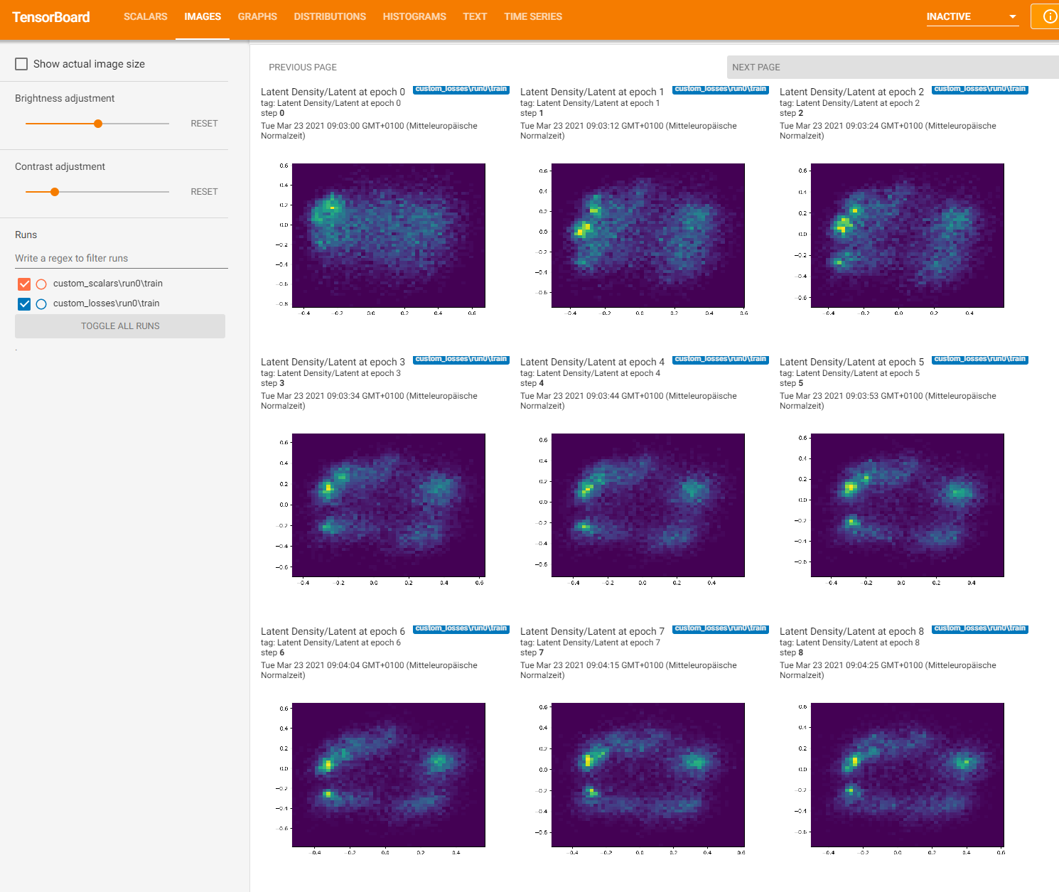
Output

Here’s what Tensorboard should put out:

Loading logs into jupyter notebook

Last but not least, we will have a look at how we could retrieve the images and logs from TensorBoard. This is not trivial, as the tfevent files, that TensorFlow writes are so-called protobuf files (for protocol buffers, a data serialization format developed by Google).

ls runs/custom_losses/run0/train

events.out.tfevents.1735476821.Marlin.415482.6.v2
events.out.tfevents.1735476821.Marlin.415482.7.v2

from tensorflow.python.summary.summary_iterator import summary_iterator
from io import BytesIO
from plotly.subplots import make_subplots
import base64
from pathlib import Path

records_files = list(
    Path(parameters.main_path).rglob("*tfevents*")
)

prefix = "data:image/png;base64,"

visited_tags = {}
image_steps = [0, 68, 399]
images_at_steps = {}

for records_file in records_files:
    visited_tags[records_file] = set()
    for i, summary in enumerate(summary_iterator(str(records_file))):
        for j, v in enumerate(summary.summary.value):
            visited_tags[records_file].add(v.tag)
            if v.tag == "Latent Output/Latent Density":
                b = tf.make_ndarray(v.tensor)[-1]
                stream = BytesIO(b)
                base64_string = prefix + base64.b64encode(stream.getvalue()).decode("utf-8")
                images_at_steps[summary.step] = base64_string

fig = make_subplots(cols=3, rows=1, subplot_titles=["step 0", "step 12", "step 67"])
fig.add_trace(
    go.Image(source=images_at_steps[0]), col=1, row=1,
)
fig.add_trace(
    go.Image(source=images_at_steps[12]), col=2, row=1,
)
fig.add_trace(
    go.Image(source=images_at_steps[67]), col=3, row=1,
)

Conclusion

Using the closure method, you can easily add new loss functions to EncoderMap.

References

@article{ceriotti2011simplifying,
  title={Simplifying the representation of complex free-energy landscapes using sketch-map},
  author={Ceriotti, Michele and Tribello, Gareth A and Parrinello, Michele},
  journal={Proceedings of the National Academy of Sciences},
  volume={108},
  number={32},
  pages={13023--13028},
  year={2011},
  publisher={National Acad Sciences}
}

@article{sawade2023combining,
  title={Combining molecular dynamics simulations and scoring method to computationally model ubiquitylated linker histones in chromatosomes},
  author={Sawade, Kevin and Marx, Andreas and Peter, Christine and Kukharenko, Oleksandra},
  journal={PLoS Computational Biology},
  volume={19},
  number={8},
  pages={e1010531},
  year={2023},
  publisher={Public Library of Science San Francisco, CA USA}
}

@article{franke2023visualizing,
  title={Visualizing the residue interaction landscape of proteins by temporal network embedding},
  author={Franke, Leon and Peter, Christine},
  journal={Journal of Chemical Theory and Computation},
  volume={19},
  number={10},
  pages={2985--2995},
  year={2023},
  publisher={ACS Publications}
}