Publication Figure 1#
This jupyter notebook contains the Analysis code for an upcoming publication.
Authors: Kevin Sawade (kevin.sawade@uni-konstanz.de), Tobias Lemke, Christine Peter (christine.peter@uni-konstanz.de)
EncoderMap’s featurization was inspired by the (no longer maintained) PyEMMA library. Consider citing it (https://dx.doi.org/10.1021/acs.jctc.5b00743), if you are using EncoderMap:
Imports#
We start with the imports.
[1]:
# Future imports at the top
from __future__ import annotations
# Import EncoderMap
import encodermap as em
from encodermap.plot import plotting
from encodermap.plot.plotting import _plot_free_energy
# Builtin packages
import re
import io
import warnings
import os
import json
import contextlib
import time
from copy import deepcopy
from types import SimpleNamespace
from pathlib import Path
# Math
import numpy as np
import pandas as pd
import xarray as xr
# ML
import tensorflow as tf
# Plotting
import plotly.express as px
import plotly.graph_objects as go
import plotly.io as pio
from plotly.subplots import make_subplots
import plotly.io as pio
# MD
import mdtraj as md
import MDAnalysis as mda
import nglview as nv
# dates
from dateutil import parser
/home/kevin/git/encoder_map_private/encodermap/__init__.py:194: GPUsAreDisabledWarning: EncoderMap disables the GPU per default because most tensorflow code runs with a higher compatibility when the GPU is disabled. If you want to enable GPUs manually, set the environment variable 'ENCODERMAP_ENABLE_GPU' to 'True' before importing EncoderMap. To do this in python you can run:
import os; os.environ['ENCODERMAP_ENABLE_GPU'] = 'True'
before importing encodermap.
_warnings.warn(
Using Autoreload we can make changes in the EncoderMap source code and use the new code, without needing to restart the Kernel.
[2]:
%load_ext autoreload
%autoreload 2
Trained network weights#
EncoderMap’s Neural Network is initialized with random weights and biases. While the training is deterministic with pre-defined training weights, and the inferences that can be made from two trained models are qualitatively similar, the numerical exact output depends on the starting weights.
For this reason, the trained network weights are available from the corresponding authors upon reasonable request or by raising an issue on GitHub: AG-Peter/encodermap#issues
The creation of this figure demonstrates three capabilities in EncoderMap:
MD Trajectory pipelines for loading, featurization, and (out-of-memory) data streaming.
Visualization of the latent space during training.
Customization of these latent space images.
The MD simulations were initially conducted in this study:
@article{10.1371/journal.pcbi.1010531,
doi = {10.1371/journal.pcbi.1010531},
author = {Sawade, Kevin AND Marx, Andreas AND Peter, Christine AND Kukharenko, Oleksandra},
journal = {PLOS Computational Biology},
publisher = {Public Library of Science},
title = {Combining molecular dynamics simulations and scoring method to computationally model ubiquitylated linker histones in chromatosomes},
year = {2023},
month = {08},
volume = {19},
url = {https://doi.org/10.1371/journal.pcbi.1010531},
pages = {1-24},
}
Load MD data from KonDATA#
The MD simulations can be obtained from the University of Konstanz’s data repository KonDATA:
https://dx.doi.org/10.48606/99
EncoderMap offers a convenient function for downloading data from KonDATA. But first, we need to define where to put the output. We will start from the Path this Jupyter-Notebook runs (Path.cwd()) and write into a analysis/images_during_training directory.
[3]:
figure_1_data_dir = Path.cwd() / "analysis/figure_1"
if not figure_1_data_dir.exists():
figure_1_data_dir.mkdir(parents=True)
EncoderMap allows direct access to Datasets on KonData (if the selenium Python package is installed).
[5]:
em.get_from_kondata(
"H1Ub",
figure_1_data_dir,
silence_overwrite_message=True,
mk_parentdir=True,
)
[5]:
'/home/kevin/git/encoder_map_private/docs/source/notebooks/publication/analysis/figure_1'
Add collective variables to MD data by featurization#
Next, we can use EncoderMap’s new data loading and featurization module to get a container of the MD data we just downloaded. This new container allows us to save a whole trajectory ensemble into a single .h5 file. This allows us to cache the analysis result and save time, the next time we do something with the trajetcory ensemble. Let us define thif file path.
[6]:
H1Ub_trajs_file = figure_1_data_dir / "trajs.h5"
And then run this Analysis script to collect the necessary data.
[7]:
if not H1Ub_trajs_file.is_file():
def match(file: Path) -> bool:
"""Function, that takes in a filename and returns a boolean,
based on whether that filename was an initial simulation (True)
or an expansion (False). See
https://doi.org/10.1371/journal.pcbi.1010531 for info about
expansions. Here, we are only interested in initial simulations
and use this function with the ``filter`` function.
This is done by counting underscore characters in a filename.
Regular files in this dataset are named for the ubiquitination
site and the chi3 angle set in the starting structure
(K30_20.xtc, K41_40.xtc, etc.). Further underscores in the filename
refer to the times, where the parent trajectory was used for
an expansion (K30_20_750_20000.xtc) was started from
the 20.000 ps frame of K30_20_750.xtc, which itself was started from
the 750 ps frame of K30_20.xtc). Some files contain the pdb code
1GHC, which needs to be accounter for.
Args:
file: The filename.
Returns:
bool: True, when filename is from an initial simulation.
"""
name = file.stem
count = 1
if "None" in name:
count += 1
if "1GHC" in name:
count += 1
return name.count("_") == count
# Common strings
common_str = ["K30", "K41", "K47", "K51", "K56", "K63"]
# The traj files
traj_files = list(output_dir.rglob("*.xtc"))
print(f"Found {len(traj_files)} `.xtc` files in the directory {output_dir}.")
# and filter them using the `match` function.
traj_files = list(
filter(
match,
traj_files,
)
)
print(f"Of these files {len(traj_files)} are from initial simulations.")
# The top files are collected by iterating over all `traj_files`
top_files = []
for file in traj_files:
# the ubq site can be extracted by string manipulation
ubq_site = re.findall(r"K\d{2}", str(file))[0]
# We use the tpr file of the 20 degree rotation for the
# topology. As the topology does not include the conformation
# we can do this
tpr_file = output_dir / f"{ubq_site}/tpr_files/{ubq_site}_20.tpr"
if not tpr_file.is_file():
tpr_file = output_dir / f"{ubq_site}/tpr_files/{ubq_site}_20_None.tpr"
# There are also `.pdb` files, which are also matched to the simulation files
nosolv_top_file = output_dir / f"{ubq_site}/nosolv_top/{file.stem}.pdb"
# if the nosolv.pdb does not exist, we
# can create it with MDAnalysis
if not nosolv_top_file.is_file():
nosolv_top_file.parent.mkdir(exist_ok=True)
assert tpr_file.is_file(), f"{tpr_file=}"
# load the tpr file
with warnings.catch_warnings():
warnings.simplefilter("ignore")
u = mda.Universe(str(tpr_file))
# create a sub-universe
u_protein = mda.Merge(u.select_atoms("not resname SOL and not resname NA and not resname CL"))
# get the coordinates from the traj file
u = mda.Universe(str(file))
coordinates = u.trajectory[0].positions
# load the coordinates into the sub-universe
u = u_protein.load_new(coordinates, format=mda.coordinates.memory.MemoryReader)
# write
with warnings.catch_warnings():
warnings.simplefilter("ignore")
with mda.Writer(nosolv_top_file) as W:
W.write(u)
assert nosolv_top_file.is_file()
# now we can append the topology files
# to the trajectory files
top_files.append(nosolv_top_file)
# Instantiate
H1Ub_trajs = em.TrajEnsemble(
trajs=traj_files,
tops=top_files,
common_str=common_str,
)
print(H1Ub_trajs)
# EncoderMap uses MDTraj when loading the files
# due to the non-standard residues LYQ and GLQ
# we need to remove some erroneous connection
# between GLQ76 and MET78 (which is MET1) of
# the substrate histone protein. We also need
# to add extra topologicalfor the LYQ-GLQ residues
# and the connection between them. This is
# dine via a dictionary specifying bonds
# and dihedral angles.
connections = {}
custom_aas = {}
# the custom amino acids and the isopeptide connections
# are unique to the different linkage sites, so they
# are dicts with str as keys and we iterate over the
# `common_str` list grouping the trajectories by their
# linkage sites
for cs in common_str:
connections[cs] = {}
for a in H1Ub_trajs.trajs_by_common_str[cs][0].top.atoms:
if a.residue.resSeq == 76 and a.name == "C":
connections[cs]["iso"] = a.index
if a.residue.resSeq == 77 and a.name == "N":
connections[cs]["del"] = a.index
for cs in common_str:
custom_aas[(cs, "LYQ")] = (
"K",
{
"optional_bonds": [ # the bonds are defined as a list of tuples
("-C", "N"), # the peptide bond to the previous aa
("N", "CA"),
("N", "H"),
("CA", "C"),
("C", "O"),
("CA", "CB"),
("CB", "CG"),
("CG", "CD"),
("CD", "CQ"),
("CQ", "NQ"),
("NQ", "HQ"),
("NQ", connections[cs]["iso"]), # the isopeptide bond to atom index 758 (GLQ-75 C)
("C", "+N"), # the peptide bond to the next aa
],
"CHI1": ["N", "CA", "CB", "CG"], # LYQ-123 has special atom names
"CHI2": ["CA", "CB", "CG", "CD"], # for its chi angles, so we define
"CHI3": ["CB", "CG", "CD", "CQ"], # them here, so they can be picked
"CHI4": ["CG", "CD", "CQ", "NQ"], # up by the featurizer
}
)
custom_aas[(cs, "GLQ")] = (
"G",
{
"optional_bonds": [
("-C", "N"), # the peptide bond to the previous aa
("N", "CA"),
("N", "H"),
("CA", "C"),
("C", "O"),
],
"delete_bonds": [
("C", connections[cs]["del"]) # remove the automatically generated bond to MET1 (MET-76) of the 2nd Ubi unit
],
"PHI": ["-C", "N", "CA", "C"], # GLQ-75 only takes part in a phi angle, not in psi or omega.
"PSI": "delete",
"OMEGA": "delete",
}
)
# in case we are re-running the
# analysis, we delete the old
# molecular features
H1Ub_trajs.del_featurizer()
H1Ub_trajs.del_CVs()
class SASA_dists(em.features.CustomFeature):
"""Subclass of EncoderMap's CustomFeature.
This class extracts the pairwise distances between solvent-accessible
surface atoms (SASA) of a ubiquitylated H1 protein. See
https://doi.org/10.1371/journal.pcbi.1010531 for more info.
The feature has 304 entries.
"""
_dim = 304
def __init__(self, trajs: em.TrajEnsemble) -> None:
"""Instantiate the class.
This instantiates the class and defines the ``self.atom_pairs``
instance attribute, which is used in the ``call()`` method.
Args:
trajs: The ``TrajEnsemble`` to load the data from.
"""
# hard-coded histon and ubiquitin residue indices
# in this counting, the histone subunit's atoms
# have higher numbers than that of Ubiquitin
# fmt: off
histon_residue_numbers = [
76, 83, 87, 93, 94,
95, 96, 105, 112, 115,
116, 120, 126, 131, 136,
138, 140, 147, 150,
]
ubi_residue_numbers = [
10, 15, 23, 31, 32,
41, 47, 48, 53, 59,
61, 62, 63, 71, 72,
73,
]
# fmt: on
# these dicts will contain the integer
# 0-based atom indices used for the SASA calculations
# as the LYQ non-standard AA can appear at different
# locations in topology, the atom numbers are not
# consistent between linkage sites. The 0-based
# residue indices are consistent.
histon_resids = {}
ubi_resids = {}
for top in trajs.top:
for resid in histon_residue_numbers + ubi_residue_numbers:
atoms = list(top.residue(resid).atoms)
filtered_atoms = [a for a in atoms if a.name == "CA"]
assert len(filtered_atoms) == 1 # make sure we only have one CA atom
CA_atom = filtered_atoms[0]
if resid in histon_residue_numbers:
histon_resids.setdefault(top, []).append(CA_atom.index)
elif resid in ubi_residue_numbers:
ubi_resids.setdefault(top, []).append(CA_atom.index)
# `self.atom` contains all H1-Ubi pairs
# these are, again, unique per linkage site, so we need
# three for loops.
self.atom_pairs = {}
for top in trajs.top:
for h in histon_resids[top]:
for u in ubi_resids[top]:
self.atom_pairs.setdefault(top, []).append(
(h, u)
)
self.atom_pairs[top] = np.asarray(self.atom_pairs[top])
self.desc = "SASA_distance"
def call(self, traj):
"""Called from the TrajEnsemble's featurizer.
Uses MDTraj's compute_distance to compute the
distances of a trajectory while upholding the minimum
image convention.
Args:
traj: An instance of encodermap.SingleTraj.
"""
dists = md.compute_distances(
traj=traj,
atom_pairs=self.atom_pairs[traj.top],
periodic=False,
)
return dists
class COG_dists(em.features.CustomFeature):
"""Calculates the center of gravity (cog) between the two subunits.
This calculation does not depend on the type of linkage and thus
can be exclusively carried out in the `call()` method.
"""
_is_custom = True
def __init__(self, trajs):
self._dim = 1
self.desc = "COG_distance"
def call(self, traj):
proximal = md.compute_center_of_geometry(traj.atom_slice(traj.top.select("backbone and resid < 76")))
distal = md.compute_center_of_geometry(traj.atom_slice(traj.top.select("backbone and resid >= 76")))
xyz = np.stack([proximal, distal], axis=1)
# Using SimpleNamespace we can trick
# MDTraj's compute_distances to accept
# the xyz coordinates of the COGs and calculate
# distances while upholding the minimum image
# convention. Otherwise, we would need to implement
# out own MIC code.
traj = SimpleNamespace(
xyz=xyz,
unitcell_lengths=traj.unitcell_lengths,
unitcell_angles=traj.unitcell_angles,
unitcell_vectors=traj.unitcell_vectors,
top=None,
)
dists = md.compute_distances(traj, atom_pairs=[[0, 1]])
return dists
# this featurization is inspired by the
# no longer maintained PyEMMA library.
# It implements custom logic to also
# allow out-of memory featurization using
# the dask distributed computing library
f = SASA_dists(H1Ub_trajs)
H1Ub_trajs.featurizer.add_custom_feature(f)
f2 = COG_dists(H1Ub_trajs)
H1Ub_trajs.featurizer.add_custom_feature(f2)
# the results of the featurization will be
# added to a trajectorie's collective variables.
H1Ub_trajs.load_CVs()
# all trajs together with all the calculations we just did
# can be saved in a single file.
H1Ub_trajs.save(H1Ub_trajs_file)
else:
H1Ub_trajs = em.load(H1Ub_trajs_file)
The collective variables are available as an xarray dataset.
[8]:
H1Ub_trajs._CVs
[8]:
<xarray.Dataset>
Dimensions: (COG_DISTS: 1, SASA_DISTS: 304, frame_num: 2001, traj_name: 1,
traj_num: 126)
Coordinates:
* COG_DISTS (COG_DISTS) <U12 'COG_distance'
* SASA_DISTS (SASA_DISTS) <U13 'SASA_distance' ... 'SASA_distance'
* frame_num (frame_num) int64 0 1 2 3 4 5 ... 1995 1996 1997 1998 1999 2000
* traj_name (traj_name) <U5 'trajs'
* traj_num (traj_num) int64 0 1 2 3 4 5 6 7 ... 119 120 121 122 123 124 125
time (traj_num, frame_num) float32 0.0 50.0 100.0 ... nan nan nan
Data variables:
COG_dists (traj_num, frame_num, COG_DISTS) float32 3.081 3.111 ... nan nan
SASA_dists (traj_num, frame_num, SASA_DISTS) float32 3.901 4.569 ... nan
Attributes:
feature_axes: ['COG_DISTS', 'SASA_DISTS']
full_paths: ['/home/kevin/encodermap_paper_images/analysis/images_du...
length_units: nm
time_units: ps
topology_files: ['/home/kevin/encodermap_paper_images/analysis/images_du...Create a TensorFlow dataset#
They can be used as a TensorFlow dataset like so:
[9]:
ds = H1Ub_trajs.tf_dataset(256, CV_names=["SASA_dists"])
ds
[9]:
<_PrefetchDataset element_spec=TensorSpec(shape=(256, 304), dtype=tf.float32, name=None)>
Now we can train EncoderMap using the dataset. First, we instantiate a Parameters class, that holds the necessary parameters for the NN training.
[10]:
p = em.Parameters(
dist_sig_parameters = (6, 10, 3, 6, 2, 3),
main_path = em.misc.run_path(figure_1_data_dir / "runs"),
tensorboard=True,
periodicity=float("inf"),
n_steps=2000,
summary_step=10,
checkpoint_step=10,
)
The parameters contain built-in help by calling .parameters
[11]:
print(p.parameters)
Parameter | Value | Description
--------------------------+--------------------------+---------------------------------------------------
n_neurons | [128, 128, 2] | List containing number of neurons for each layer
| | up to the bottleneck layer. For example [128, 128,
| | 2] stands for an autoencoder with the following
| | architecture {i, 128, 128, 2, 128, 128, i} where i
| | is the number of dimensions of the input data.
| | These are Input/Output Layers that are not
| | trained.
--------------------------+--------------------------+---------------------------------------------------
activation_functions | ['', 'tanh', 'tanh', ''] | List of activation function names as implemented
| | in TensorFlow. For example: "relu", "tanh",
| | "sigmoid" or "" to use no activation function. The
| | encoder part of the network takes the activation
| | functions from the list starting with the second
| | element. The decoder part of the network takes the
| | activation functions in reversed order starting
| | with the second element form the back. For example
| | ["", "relu", "tanh", ""] would result in a
| | autoencoder with {"relu", "tanh", "", "tanh",
| | "relu", ""} as sequence of activation functions.
--------------------------+--------------------------+---------------------------------------------------
periodicity | inf | Defines the distance between periodic walls for
| | the inputs. For example 2pi for angular values in
| | radians. All periodic data processed by EncoderMap
| | must be wrapped to one periodic window. E.g. data
| | with 2pi periodicity may contain values from -pi
| | to pi or from 0 to 2pi. Set the periodicity to
| | float("inf") for non-periodic inputs.
--------------------------+--------------------------+---------------------------------------------------
learning_rate | 0.001 | Learning rate used by the optimizer.
--------------------------+--------------------------+---------------------------------------------------
n_steps | 2000 | Number of training steps.
--------------------------+--------------------------+---------------------------------------------------
batch_size | 256 | Number of training points used in each training
| | step
--------------------------+--------------------------+---------------------------------------------------
summary_step | 10 | A summary for TensorBoard is writen every
| | summary_step steps.
--------------------------+--------------------------+---------------------------------------------------
checkpoint_step | 10 | A checkpoint is writen every checkpoint_step
| | steps.
--------------------------+--------------------------+---------------------------------------------------
dist_sig_parameters | (6, 10, 3, 6, 2, 3) | Parameters for the sigmoid functions applied to
| | the high- and low-dimensional distances in the
| | following order (sig_h, a_h, b_h, sig_l, a_l, b_l)
--------------------------+--------------------------+---------------------------------------------------
distance_cost_scale | 500 | Adjusts how much the distance based metric is
| | weighted in the cost function.
--------------------------+--------------------------+---------------------------------------------------
auto_cost_scale | 1 | Adjusts how much the autoencoding cost is weighted
| | in the cost function.
--------------------------+--------------------------+---------------------------------------------------
auto_cost_variant | mean_abs | defines how the auto cost is calculated. Must be
| | one of: * `mean_square` * `mean_abs` * `mean_norm`
--------------------------+--------------------------+---------------------------------------------------
center_cost_scale | 0.0001 | Adjusts how much the centering cost is weighted in
| | the cost function.
--------------------------+--------------------------+---------------------------------------------------
l2_reg_constant | 0.001 | Adjusts how much the L2 regularisation is weighted
| | in the cost function.
--------------------------+--------------------------+---------------------------------------------------
gpu_memory_fraction | | Specifies the fraction of gpu memory blocked. If
| | set to 0, memory is allocated as needed.
--------------------------+--------------------------+---------------------------------------------------
analysis_path | | A path that can be used to store analysis
--------------------------+--------------------------+---------------------------------------------------
id | | Can be any name for the run. Might be useful for
| | example for specific analysis for different data
| | sets.
--------------------------+--------------------------+---------------------------------------------------
model_api | sequential | A string defining the API to be used to build the
| | keras model. Defaults to `sequntial`. Possible
| | strings are: * `functional` will use keras'
| | functional API. * `sequential` will define a keras
| | Model, containing two other models with the
| | Sequential API. These two models are encoder and
| | decoder. * `custom` will create a custom Model
| | where even the layers are custom.
--------------------------+--------------------------+---------------------------------------------------
loss | emap_cost | A string defining the loss function. Defaults to
| | `emap_cost`. Possible losses are: *
| | `reconstruction_loss` will try to train output ==
| | input * `mse`: Returns a mean squared error loss.
| | * `emap_cost` is the EncoderMap loss function.
| | Depending on the class `Autoencoder`, `Encodermap,
| | `ADCAutoencoder`, different contributions are used
| | for a combined loss. Autoencoder uses atuo_cost,
| | reg_cost, center_cost. EncoderMap class adds
| | sigmoid_loss.
--------------------------+--------------------------+---------------------------------------------------
training | auto | A string defining what kind of training is
| | performed when autoencoder.train() is callsed. *
| | `auto` does a regular model.compile() and
| | model.fit() procedure. * `custom` uses gradient
| | tape and calculates losses and gradients manually.
--------------------------+--------------------------+---------------------------------------------------
batched | True | Whether the dataset is batched or not.
--------------------------+--------------------------+---------------------------------------------------
tensorboard | True | Whether to print tensorboard information. Defaults
| | to False.
--------------------------+--------------------------+---------------------------------------------------
seed | | Fixes the state of all operations using random
| | numbers. Defaults to None.
--------------------------+--------------------------+---------------------------------------------------
current_training_step | | The current training step. Aids in reloading of
| | models.
--------------------------+--------------------------+---------------------------------------------------
write_summary | | If True writes a summar.txt of the models into
| | main_path if `tensorboard` is True, summaries will
| | also be written.
--------------------------+--------------------------+---------------------------------------------------
trainable_dense_to_sparse | | When using different topologies to train the
| | AngleDihedralCartesianEncoderMap, some inputs
| | might be sparse, which means, they have missing
| | values. Creating a dense input is done by first
| | passing these sparse tensors through
| | `tf.keras.layers.Dense` layers. These layers have
| | trainable weights, and if this parameter is True,
| | these weights will be changed by the optimizer.
--------------------------+--------------------------+---------------------------------------------------
using_hypercube | | This parameter is not meant to be set by the user.
Now, we can instantiate the EncoderMap class.
[13]:
e_map = em.EncoderMap(
parameters=p,
train_data=ds,
)
Output files are saved to /home/kevin/git/encoder_map_private/docs/source/notebooks/publication/analysis/figure_1/runs/run16 as defined in 'main_path' in the parameters.
Saved a text-summary of the model and an image in /home/kevin/git/encoder_map_private/docs/source/notebooks/publication/analysis/figure_1/runs/run16, as specified in 'main_path' in the parameters.
Using the save() method, we can also save the initial weights of the model.
[14]:
e_map.save(0)
Saving the model to /home/kevin/git/encoder_map_private/docs/source/notebooks/publication/analysis/figure_1/runs/run16/saved_model_0.keras. Use `em.EncoderMap.from_checkpoint('/home/kevin/git/encoder_map_private/docs/source/notebooks/publication/analysis/figure_1/runs/run16')` to load the most recent model, or `em.EncoderMap.from_checkpoint('/home/kevin/git/encoder_map_private/docs/source/notebooks/publication/analysis/figure_1/runs/run16/saved_model_0.keras')` to load the model with specific weights..
This model has a subclassed encoder, which can be loaded independently. Use `tf.keras.load_model('/home/kevin/git/encoder_map_private/docs/source/notebooks/publication/analysis/figure_1/runs/run16/saved_model_0_encoder.keras')` to load only this model.
This model has a subclassed decoder, which can be loaded independently. Use `tf.keras.load_model('/home/kevin/git/encoder_map_private/docs/source/notebooks/publication/analysis/figure_1/runs/run16/saved_model_0_decoder.keras')` to load only this model.
[14]:
PosixPath('/home/kevin/git/encoder_map_private/docs/source/notebooks/publication/analysis/figure_1/runs/run16')
Plot images during training#
Saving images during the run can be enables by calling add_images_to_tensorboard.
We can also add custom colorations by creating some functions. For that, we first need to get some example data from the trajectories. This example data needs to be smaller than the complete dataset, which encompasses 126 trajectories with 2000 frames each. We use the subsample() method of the TrajEnsemble object to extract every 100th frame of the simulations.
[15]:
subsample = H1Ub_trajs.subsample(100)
plotting_data = subsample.CVs["SASA_dists"]
[16]:
plotting_data.shape
[16]:
(678, 304)
Now we can define the plotting functions. Refer to EncoderMap’s tutorials to write your own plotting functions.
[17]:
cogs = subsample.CVs["COG_dists"]
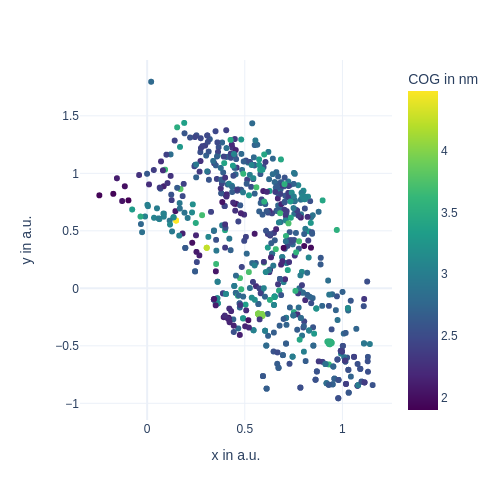
def plot_cog(lowd, color=cogs):
"""Takes in the current low-dimensional data of the latent units
and returns a tf.Tensor, that can be interpreted by `tf.summary.image_summary()`.
"""
x, y = lowd.T
# actual plotting
fig = px.scatter(
x=x,
y=y,
color=color,
color_continuous_scale="Viridis",
labels={
"x": "x in a.u.",
"y": "y in a.u.",
"color": "COG in nm",
},
width=500,
height=500,
)
# BytesIO
buf = io.BytesIO()
fig.write_image(buf)
buf.seek(0)
# tensorflow
image = tf.image.decode_png(buf.getvalue(), 4) # 4 is due to RGBA colors.
image = tf.expand_dims(image, 0)
return image
traj_nums = []
for traj_num, frame_num, frame in subsample.iterframes():
traj_nums.append(traj_num)
traj_nums = np.asarray(traj_nums)
def plot_traj_num(lowd, color=traj_nums):
"""Takes in the current low-dimensional data of the latent units
and returns a tf.Tensor, that can be interpreted by `tf.summary.image_summary()`.
"""
x, y = lowd.T
# actual plotting
fig = px.scatter(
x=x,
y=y,
color=color,
color_continuous_scale="Viridis",
labels={
"x": "x in a.u.",
"y": "y in a.u.",
"color": "traj num",
},
width=500,
height=500,
)
# BytesIO
buf = io.BytesIO()
fig.write_image(buf)
buf.seek(0)
# tensorflow
image = tf.image.decode_png(buf.getvalue(), 4) # 4 is due to RGBA colors.
image = tf.expand_dims(image, 0)
return image
ubq_sites = []
ubq_sites_matches = {
"K30": 0,
"K41": 1,
"K47": 2,
"K51": 3,
"K56": 4,
"K63": 5,
}
for traj_num, frame_num, frame in subsample.iterframes():
ubq_sites.append(ubq_sites_matches[frame.common_str])
ubq_sites = np.asarray(ubq_sites)
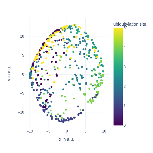
def plot_ubq_site(lowd, color=ubq_sites):
"""Takes in the current low-dimensional data of the latent units
and returns a tf.Tensor, that can be interpreted by `tf.summary.image_summary()`.
"""
x, y = lowd.T
# actual plotting
fig = px.scatter(
x=x,
y=y,
color=color,
color_continuous_scale="Viridis",
labels={
"x": "x in a.u.",
"y": "y in a.u.",
"color": "ubiquitylation site",
},
width=500,
height=500,
)
# BytesIO
buf = io.BytesIO()
fig.write_image(buf)
buf.seek(0)
# tensorflow
image = tf.image.decode_png(buf.getvalue(), 4) # 4 is due to RGBA colors.
image = tf.expand_dims(image, 0)
return image
[18]:
e_map.add_images_to_tensorboard(
data=plotting_data,
save_to_disk=True,
additional_fns=[plot_cog, plot_traj_num, plot_ubq_site],
)
Logging images with (678, 304)-shaped data every 10 epochs to Tensorboard at /home/kevin/git/encoder_map_private/docs/source/notebooks/publication/analysis/figure_1/runs/run16
Train / load trained network#
The network provided by EncoderMap can now be trained.
(For maximum compatibility, the matrix weights of the model are provided in weights_raw.json).
[20]:
figure_1_trained_nn_dir = Path.cwd() / "trained_networks/figure_1"
if input(
"Train a network (y) or load a trained network datasets?"
) == "y":
e_map.train()
with open(figure_1_trained_nn_dir / "weights_raw.json", "w") as f:
json.dump([i.tolist() for i in emap.model.get_weights()], f)
else:
emap = em.EncoderMap.from_checkpoint(
figure_1_trained_nn_dir,
)
Train a network (y) or load a trained network datasets?
Seems like the parameter file was moved to another directory. Parameter file is updated ...
Output files are saved to /home/kevin/git/encoder_map_private/docs/source/notebooks/publication/trained_networks/figure_1 as defined in 'main_path' in the parameters.
Saved a text-summary of the model and an image in /home/kevin/git/encoder_map_private/docs/source/notebooks/publication/trained_networks/figure_1, as specified in 'main_path' in the parameters.
Look at the images that have been saved during training#
The images can be found in the training folder and viewed using the display() function and Image class from IPython.
[21]:
from IPython.display import Image, display
display(Image(figure_1_trained_nn_dir / "train_images/epoch_0_user_fn_0.png", width=600))
[22]:
from IPython.display import Image, display
display(Image(figure_1_trained_nn_dir / "train_images/epoch_50_user_fn_2.png", width=600))
Final image#
The final image which combines and highlights the importance of these additions can be constructed like so.
[23]:
steps = [0, 10, 50, 300, 2000]
titles = [f"step {s}" for s in steps]
fig = make_subplots(
cols=len(steps),
rows=3,
subplot_titles=titles,
# specs=[[{}, {}]],
horizontal_spacing=0.05,
vertical_spacing=0.05
)
# traj_nums
for i, step in enumerate(steps):
emap_instance = em.EncoderMap.from_checkpoint(
figure_1_trained_nn_dir / f"saved_model_{step}.keras",
use_previous_model=True,
)
lowd = emap_instance.encode(H1Ub_trajs.CVs["SASA_dists"])
fig.add_trace(
go.Scattergl(
x=lowd[:, 0],
y=lowd[:, 1],
mode="markers",
showlegend=False,
marker_color=H1Ub_trajs.id[:, 0],
marker_colorscale="Viridis",
marker_coloraxis="coloraxis1",
marker_size=3,
marker_opacity=0.5,
),
row=1,
col=i+1
)
# cog distance
fig.add_trace(
go.Scattergl(
x=lowd[:, 0],
y=lowd[:, 1],
mode="markers",
showlegend=False,
marker_color=H1Ub_trajs.CVs["COG_dists"],
marker_colorscale="Viridis",
marker_coloraxis="coloraxis2",
marker_size=3,
marker_opacity=0.5,
),
row=2,
col=i+1
)
# common_str
plotly_colors = [
"rgb(31, 119, 180)",
"rgb(255, 127, 14)",
"rgb(44, 160, 44)",
"rgb(214, 39, 40)",
"rgb(148, 103, 189)",
"rgb(140, 86, 75)",
"rgb(227, 119, 194)",
]
colors = []
for traj in H1Ub_trajs:
index = H1Ub_trajs.common_str.index(traj.common_str)
colors.extend([index for i in range(traj.n_frames)])
fig.add_trace(
go.Scattergl(
x=lowd[:, 0],
y=lowd[:, 1],
mode="markers",
showlegend=False,
marker_color=colors,
marker_colorscale="Viridis",
marker_coloraxis="coloraxis3",
marker_size=3,
marker_opacity=0.5,
),
row=3,
col=i+1
)
showstuff = False
fig.for_each_xaxis(lambda x: x.update(showgrid=showstuff, showline=showstuff, zeroline=showstuff, showticklabels=showstuff))
fig.for_each_yaxis(lambda x: x.update(showgrid=showstuff, showline=showstuff, zeroline=showstuff, showticklabels=showstuff))
scales = {}
identifier = 1
for col in range(1, 6):
for row in range(1, 4):
scales[f"yaxis{identifier}"] = {
"scaleanchor": f"x{identifier}",
"scaleratio": 1,
}
identifier += 1
fig.update_layout(
{
"width": 1200,
"height": 800,
"paper_bgcolor": "rgba(0, 0, 0, 0)",
"plot_bgcolor": "rgba(0, 0, 0, 0)",
"coloraxis1": {
"colorscale": "Viridis",
"colorbar": {
"x": 1,
"title": "traj num",
"len": 0.3,
"y": 0.9,
"tickfont": {
"size": 14,
},
}
},
"coloraxis2": {
"colorscale": "Viridis",
"colorbar": {
"x": 1,
"title": "COG distance in nm",
"len": 0.3,
"y": 0.5,
"tickfont": {
"size": 14,
},
}
},
"margin": {
"t": 0,
"b": 0,
"r": 15,
"l": 0,
},
"coloraxis3": {
"colorscale": "Viridis",
"colorbar": {
"x": 1,
"title": "ubiquitylation site",
"len": 0.3,
"y": 0.1,
"tickvals": [0, 1, 2, 3, 4, 5],
"ticktext": ["K30", "K41", "K47", "K51", "K56", "K63"],
"tickfont": {
"size": 14,
},
}
},
} | scales,
)
for i in fig['layout']['annotations']:
i['font'] = dict(size=22)
# fig.write_image(figure_1_trained_nn_dir / "figure1.svg", scale=2)
# fig.write_image(figure_1_trained_nn_dir / "figure1.png", scale=2)
fig.show()
Seems like the parameter file was moved to another directory. Parameter file is updated ...
Output files are saved to /home/kevin/git/encoder_map_private/docs/source/notebooks/publication/trained_networks/figure_1 as defined in 'main_path' in the parameters.
Saved a text-summary of the model and an image in /home/kevin/git/encoder_map_private/docs/source/notebooks/publication/trained_networks/figure_1, as specified in 'main_path' in the parameters.