Publication Figure 3

This jupyter notebook contains the Analysis code for an upcoming publication.

Authors: Kevin Sawade (kevin.sawade@uni-konstanz.de), Christine Peter (christine.peter@uni-konstanz.de)

EncoderMap’s featurization was inspired by the (no longer maintained) PyEMMA library. Consider citing it (https://dx.doi.org/10.1021/acs.jctc.5b00743), if you are using EncoderMap.

This notebook was revised upon the request of a reviewer.

Imports

We start with the imports.

# Future imports at the top
from __future__ import annotations

# Import EncoderMap
import encodermap as em
from encodermap.plot import plotting
from encodermap.plot.plotting import _plot_free_energy

# Builtin packages
import re
import io
import warnings
import os
import json
import contextlib
import time
from copy import deepcopy
from types import SimpleNamespace
from pathlib import Path

# Math
import numpy as np
import pandas as pd
import xarray as xr

# ML
import tensorflow as tf
from sklearn.decomposition import PCA

# Plotting
import plotly.express as px
import plotly.graph_objects as go
import plotly.io as pio
from plotly.subplots import make_subplots
import plotly.io as pio

# MD
import mdtraj as md
import MDAnalysis as mda
import nglview as nv

# dates
from dateutil import parser

/home/kevin/git/encoder_map_private/encodermap/__init__.py:194: GPUsAreDisabledWarning: EncoderMap disables the GPU per default because most tensorflow code runs with a higher compatibility when the GPU is disabled. If you want to enable GPUs manually, set the environment variable 'ENCODERMAP_ENABLE_GPU' to 'True' before importing EncoderMap. To do this in python you can run:

import os; os.environ['ENCODERMAP_ENABLE_GPU'] = 'True'

before importing encodermap.
  _warnings.warn(

Using Autoreload we can make changes in the EncoderMap source code and use the new code, without needing to restart the Kernel.

%load_ext autoreload
%autoreload 2

Trained network weights

EncoderMap’s Neural Network is initialized with random weights and biases. While the training is deterministic with pre-defined training weights, and the inferences that can be made from two trained models are qualitatively similar, the numerical exact output depends on the starting weights.

For this reason, the trained network weights are available from the corresponding authors upon reasonable request or by raising an issue on GitHub: AG-Peter/encodermap#issues

This figure demonstrates the

1. The modularity of the EncoderMap package.

2. Some interactive elements in EncoderMap.

Get data

We will use the same data as in Figure 1. To obtain the H1Ub_trajs variable, use the cells from figure 1. We will also use the SASA_dists collective variable as the training input. For plotting, we will select a subset of the trajectory ensemble with 10000 frames.

figure_1_data_dir = Path.cwd() / "../analysis/figure_1"
if not figure_1_data_dir.exists():
    figure_1_data_dir.mkdir(parents=True)
em.get_from_kondata(
    "H1Ub",
    figure_1_data_dir,
    silence_overwrite_message=True,
    mk_parentdir=True,
)
H1Ub_trajs_file = figure_1_data_dir / "trajs.h5"
H1Ub_trajs = em.load(H1Ub_trajs_file)

This will be the output directory

figure_3_trained_nn_dir = (Path.cwd() / "../trained_networks/figure_3").resolve()

figure_3_trained_nn_dir

PosixPath('/home/kevin/encodermap_paper_images/trained_networks/figure_3')

“Classical” methods

Before delving into neural networks and machine learning we will start with some “classical” dimensionality reduction methods.

MDS

In multi-dimensional scaling (MDS) a set of \(m\) points \(P = (x \vert x \in \mathbb{R}^N)\), where \(N\) is the input dimension of the set is projected into a lower dimension \(n\) by minimizing the \(\text{Strain}_D\) function with:

\begin{equation} \text{Strain}_D(x_1, x_2, ..., x_m) = \left( \frac{\sum_{ij} \left( b_{ij} - x^T_i x_j \right)^2}{\sum_{ij} b^2_{ij}} \right)^{\frac{1}{2}} \end{equation}

The following formulas are taken from https://www.mathpsy.uni-tuebingen.de/wickelmaier/pubs/Wickelmaier2003SQRU.pdf

The solution to this problem rests on the fact, that the cooridnate matrix \(\mathbf{X}\) of all \((x_1, x_2, ..., x_m)\) can be derived by eigenvalue decomposition from the scalar product matrix \(\mathbf{B} = \mathbf{XX'}\). The problem of constructing \(\mathbf{B}\) from the proximity matrix \(\mathbf{P}\) is solved by multiplying the squared proximities with the matrix \(\mathbf{J} = \mathbf{I} - n^{-1}\mathbf{11'}\). This procedure is called double centering. The following steps summarize the algorithm of classical MDS:

0. A limit when doing MDS is the size of the memory of the computer. The memory complexity scales with \(\mathcal{O}(n^2)\). Let’s assume the array contains double precision float64 numbers with 64 bits (8 bytes) each and calculate the theoretical memory size of a 2D \(m \times m\) array holding all \(m\) points of the H1Ub dataset.

s = np.dtype(float).itemsize
print(f"A single float takes {s} bytes of memory.")
n_frames = H1Ub_trajs.n_frames
print(f"The H1Ub dataset encompasses {n_frames} frames")
bytes = s * H1Ub_trajs.n_frames** 2
print(f"The {n_frames} x {n_frames} proximity matrix has a size of {bytes} bytes.")
gb = bytes / 1024 / 1024 / 1024
print(f"This is {gb} Giga bytes.")

A single float takes 8 bytes of memory.
The H1Ub dataset encompasses 55326 frames
The 55326 x 55326 proximity matrix has a size of 24487730208 bytes.
This is 22.805975943803787 Giga bytes.

To leave some room in the memory for intermediate computations we have to select a subset of points from the “SASA_dists” (see notebook to figure 1).

subsample_file = Path.cwd() / "H1Ub_subsample.h5"

if not subsample_file.is_file():
    subsample = H1Ub_trajs.subsample(10)
    subsample.save(subsample_file)
subsample = em.load(subsample_file)

1. Set up the matrix of squared proximities: \(\mathbf{P^{(2)}} = \left[ p^2 \right]\).

from sklearn.metrics import euclidean_distances as sk_euclidean_distances

proximity_matrix = sk_euclidean_distances(subsample.SASA_dists)
print(proximity_matrix.shape)

(5646, 5646)

P = proximity_matrix ** 2

2. Apply the double centering: \(\mathbf{B} = -\frac{1}{2}\mathbf{JP^{(2)}J}\) using the matrix \(\mathbf{J} = \mathbf{I} - m^{-1}\mathbf{11'}\).

m = proximity_matrix.shape[0]
diag_one = np.eye(m)
fill_one = np.ones(m)

J = diag_one - m ** -1 * fill_one

B = - (1/2) * np.matmul(np.matmul(J, P), J)

3. Extract the \(n\) largest positive eigenvalues \(\lambda_1, ..., \lambda_n\) of \(\mathbf{B}\) and the corresponding \(n\) eigenvectors \(\mathbf{e_1}, ..., \mathbf{e_m}\).

eigen = np.linalg.eig(B)
eigen1, eigen2 = eigen[0][:2]
print(eigen1, eigen2)

(542845.4505927933+0j) (213383.93846512752+0j)

4. A \(n\)-dimensional spatial configuration of the \(m\) objects is derived from the coordinate matrix \(X = E_n\Lambda^{1/2}_n\), where \(E_n\) is the matrix of \(n\) eigenvectors and \(\Lambda_n\) is the diagonal matrix of \(n\) eigenvalues of \(B\), respectively.

two_d_eigenmatrix = eigen[1][:,:2]
X = np.matmul(two_d_eigenmatrix, np.array([[np.sqrt(eigen1), 0], [0, np.sqrt(eigen2)]])).real
subsample.load_CVs(X[:, :2], "MDS_lowd")

Extract a cluster from MDS

# subsample.del_CVs(["_user_selected_points", "lowd"])
# sess = em.InteractivePlotting(
#     trajs=subsample,
#     highd_data=subsample.CVs["SASA_dists"],
#     lowd_data=X,
# )

# (figure_3_trained_nn_dir / "MDS/clusters/cluster0/").mkdir(parents=True, exist_ok=True)
# np.save(figure_3_trained_nn_dir / "MDS/clusters/cluster0/selected_points.npy", subsample._user_selected_points)
subsample.load_CVs(
    np.load(figure_3_trained_nn_dir / "MDS/clusters/cluster0/selected_points.npy"),
    "_user_selected_points",
)
# cluster = H1Ub_trajs[subsample.id[subsample._user_selected_points == 0]]
# traj = cluster[::10].stack()
# traj.save_pdb(figure_3_trained_nn_dir / "MDS/clusters/cluster0/cluster0.pdb")

Plot

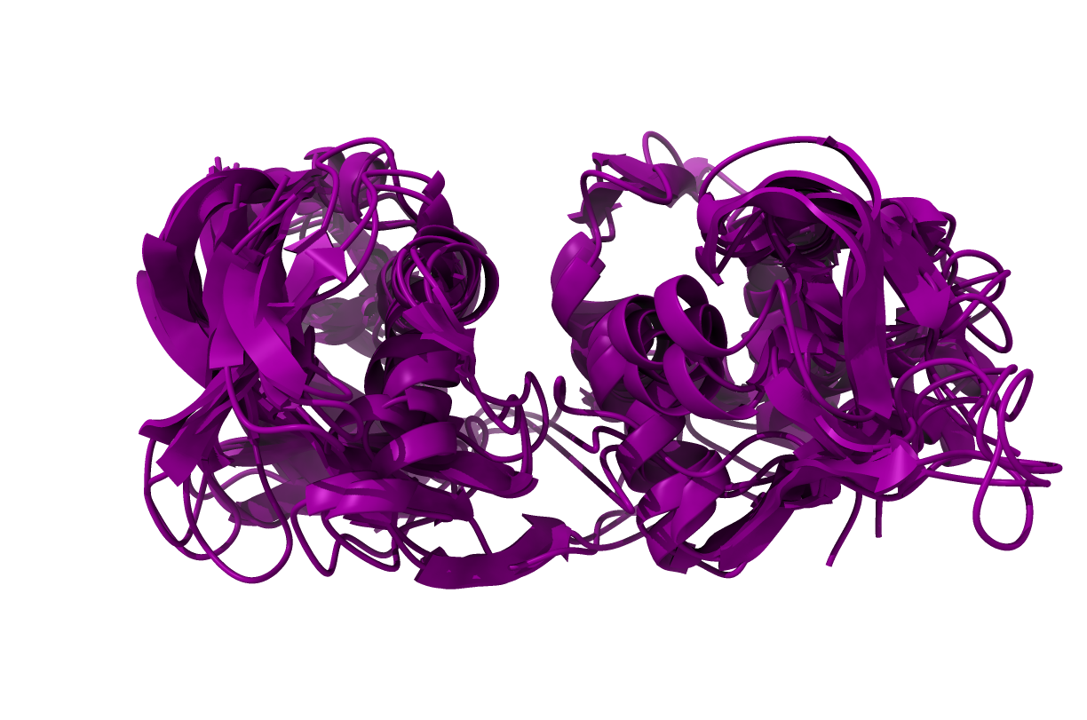
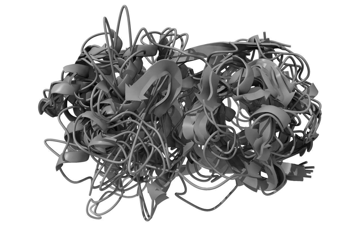
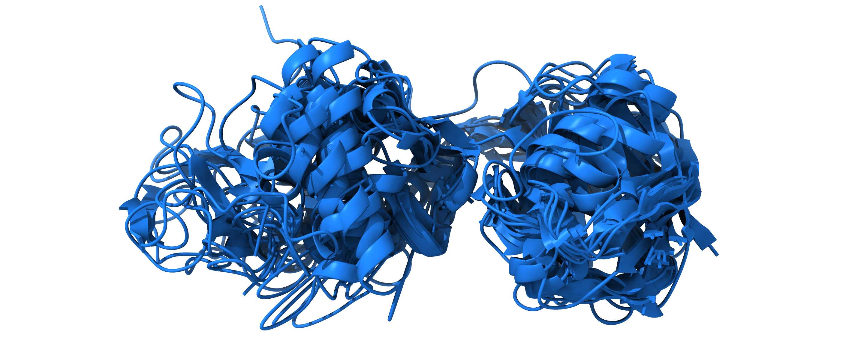
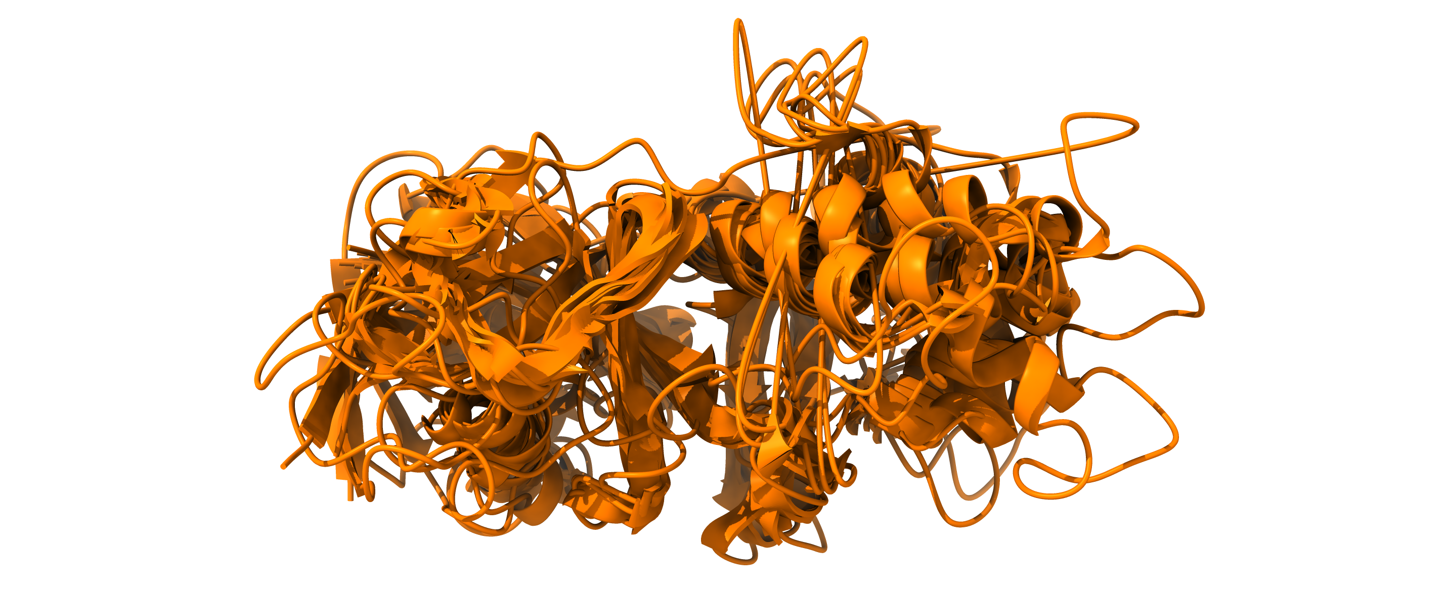
The secondary structure render in figure the figure was done using UCSF ChimeraX.

from encodermap.plot.plotting import _plot_free_energy
from PIL import Image

fig = make_subplots(
    cols=4,
    rows=1,
    subplot_titles=[
        "classical MDS", "", "highd trace", "Cluster 1",
    ],
    column_widths=[1, 1, 0.2, 1],
    horizontal_spacing=0.05,
    vertical_spacing=0.05,
)

fig.add_trace(
    _plot_free_energy(
        x=subsample.MDS_lowd[:, 0],
        y=subsample.MDS_lowd[:, 1],
        bins=35
    ),
    row=1,
    col=1,
)

fig.add_trace(
    go.Scattergl(
        x=subsample.MDS_lowd[::5, 0],
        y=subsample.MDS_lowd[::5, 1],
        marker_color="rgba(120, 120, 120, 0.1)",
        mode="markers",
        name="",
        showlegend=False,
    ),
    row=1,
    col=2,
)

cluster_lowd = subsample.MDS_lowd[subsample._user_selected_points == 0]
fig.add_trace(
    go.Scattergl(
        x=cluster_lowd[:, 0],
        y=cluster_lowd[:, 1],
        marker_color="purple",
        marker_opacity=1.0,
        marker_size=10,
        mode="markers",
        name="",
        showlegend=False,
    ),
    row=1,
    col=2,
)

# highd trace
cluster_highd = subsample.SASA_dists[subsample._user_selected_points == 0]
fig.add_trace(
    go.Heatmap(
        z=cluster_highd.T,
        showlegend=False,
        showscale=False,
        colorscale="Viridis",
        hoverinfo="skip",
        name="",
        hovertemplate="",
    ),
    row=1,
    col=3,
)

# image
image_file = figure_3_trained_nn_dir / f"MDS/clusters/cluster0/cluster_0_chimeraX_render.png"
# with Image.open(image_file) as img:
#     fig.add_trace(
#         go.Image(z=np.asarray(img)),
#         row=1,
#         col=4,
#     )

showstuff = False
fig.for_each_xaxis(lambda x: x.update(showgrid=showstuff, showline=showstuff, zeroline=showstuff, showticklabels=showstuff))
fig.for_each_yaxis(lambda x: x.update(showgrid=showstuff, showline=showstuff, zeroline=showstuff, showticklabels=showstuff))
scales = {}
identifier = 1
for row in range(1, 4):
    for col in range(1, 5):
        if col in [1, 2] and row in [1, 2, 3]:
            scales[f"yaxis{identifier}"] = {
                "scaleanchor": f"x{identifier}",
                "scaleratio": 1,
            }
        identifier += 1
fig.update_layout(
    {
        "width": 1000,
        "height": 300,
        "margin": dict(t=40, b=0, r=0, l=0),
    } | scales,
)
# fig.write_image(figure_3_trained_nn_dir / "SI_figure3_MDS.svg", scale=2)
# fig.write_image(figure_3_trained_nn_dir / "SI_figure3_MDS.png", scale=2)
fig.show()

PCA

The idea behind PCA is to achieve a corrdinate transformation of all input points and all input dimensions, so that the first and second dimensions in the transoformed space exhibit the maximal variance. The dimensions after these two are usually dropped resulting in an embedding of high to low.

The formulas in this section are taken from: https://medium.com/@nahmed3536/a-python-implementation-of-pca-with-numpy-1bbd3b21de2e

1. Standardize the Data (Optional but Common): Each variable is centered by subtracting its mean and often scaled to have unit variance, ensuring that every variable contributes equally.

data = H1Ub_trajs.SASA_dists.copy()
data.shape

(55326, 304)

standardized_data = (data - data.mean(axis = 0)) / data.std(axis = 0)
standardized_data.shape

(55326, 304)

2. Compute the Covariance Matrix:

   For the data matrix \(X\) (with rows as observations and columns as variables), the covariance matrix is calculated as
   \begin{equation} \Sigma = \frac{1}{n - 1} X^T X \end{equation}

   This matrix captures how each pair of variables varies together.

covariance_matrix = np.cov(standardized_data, ddof = 1, rowvar = False)
covariance_matrix.shape

(304, 304)

3. Compute Eigenvalues and Eigenvectors: Solve the equation \begin{equation} \Sigma v = \lambda v \end{equation} where the eigenvectors \(v\) represent the directions of the principal components, and the eigenvalues \(\lambda\) indicate the amount of variance each component explains.

eigenvalues, eigenvectors = np.linalg.eig(covariance_matrix)

4. Rank Components by Variance: Sort the eigenvalues (and their corresponding eigenvectors) in descending order. The eigenvector with the largest eigenvalue becomes the first principal component, holding the highest variance.

order_of_importance = np.argsort(eigenvalues)[::-1]
sorted_eigenvalues = eigenvalues[order_of_importance]
sorted_eigenvectors = eigenvectors[:,order_of_importance]

5. Project the Data: Form a matrix \(W\) from the top \(k\) eigenvectors and project the original data using the equation \begin{equation} Z = XW \end{equation} This projection yields a lower-dimensional representation of the data that retains most of its significant information.

explained_variance = sorted_eigenvalues / np.sum(sorted_eigenvalues)

6. **Reduce to the \(k\) principial components.

This can be done via np.matmul.

k = 2 # select the number of principal components
reduced_data = np.matmul(standardized_data, sorted_eigenvectors[:,:k])

Plot.

px.scatter(x=reduced_data[:, 0], y=reduced_data[:, 1])

SciKit Learn implementation

pca = PCA(n_components=0.99)
X = pca.fit_transform(H1Ub_trajs.SASA_dists)

X.shape

(55326, 30)

H1Ub_trajs.load_CVs(X[:, :2], "PCA_lowd")

px.scatter(x=X[:, 0], y=X[:, 1])

Extract a cluster from PCA

H1Ub_trajs.del_CVs(["_user_selected_points", "lowd"])
sess = em.InteractivePlotting(
    trajs=H1Ub_trajs,
    highd_data=H1Ub_trajs.CVs["SASA_dists"],
    lowd_data=X[:, :2],
)

# (figure_3_trained_nn_dir / "PCA/clusters/cluster0/").mkdir(parents=True, exist_ok=True)
# np.save(figure_3_trained_nn_dir / "PCA/clusters/cluster0/selected_points.npy", H1Ub_trajs._user_selected_points)
H1Ub_trajs.load_CVs(
    np.load(figure_3_trained_nn_dir / "PCA/clusters/cluster0/selected_points.npy"),
    "_user_selected_points",
)
# cluster = H1Ub_trajs.cluster(0, "_user_selected_points", n_points=10)
# traj = cluster.stack()
# traj.save_pdb(figure_3_trained_nn_dir / "PCA/clusters/cluster0/cluster0.pdb")

Plot

from encodermap.plot.plotting import _plot_free_energy
from PIL import Image

fig = make_subplots(
    cols=4,
    rows=1,
    subplot_titles=[
        "classical PCA", "", "highd trace", "Cluster 1",
    ],
    column_widths=[1, 1, 0.2, 1],
    horizontal_spacing=0.05,
    vertical_spacing=0.05,
)

lowd_data = X
fig.add_trace(
    _plot_free_energy(
        x=H1Ub_trajs.PCA_lowd[:, 0],
        y=H1Ub_trajs.PCA_lowd[:, 1],
        bins=35
    ),
    row=1,
    col=1,
)

fig.add_trace(
    go.Scattergl(
        x=H1Ub_trajs.PCA_lowd[::5, 0],
        y=H1Ub_trajs.PCA_lowd[::5, 1],
        marker_color="rgba(120, 120, 120, 0.1)",
        mode="markers",
        name="",
        showlegend=False,
    ),
    row=1,
    col=2,
)

cluster_lowd = H1Ub_trajs.PCA_lowd[H1Ub_trajs._user_selected_points == 0]

fig.add_trace(
    go.Scattergl(
        x=cluster_lowd[:, 0],
        y=cluster_lowd[:, 1],
        marker_color="darkgrey",
        marker_opacity=1.0,
        marker_size=10,
        mode="markers",
        name="",
        showlegend=False,
    ),
    row=1,
    col=2,
)

# highd trace
cluster_highd = H1Ub_trajs.SASA_dists[H1Ub_trajs._user_selected_points == 0]
fig.add_trace(
    go.Heatmap(
        z=cluster_highd.T,
        showlegend=False,
        showscale=False,
        colorscale="Viridis",
        hoverinfo="skip",
        name="",
        hovertemplate="",
    ),
    row=1,
    col=3,
)

# image
# image_file = figure_3_trained_nn_dir / f"PCA/clusters/cluster0/cluster_0_chimeraX_render.png"
# with Image.open(image_file) as img:
#     fig.add_trace(
#         go.Image(z=np.asarray(img)),
#         row=1,
#         col=4,
#     )

showstuff = False
fig.for_each_xaxis(lambda x: x.update(showgrid=showstuff, showline=showstuff, zeroline=showstuff, showticklabels=showstuff))
fig.for_each_yaxis(lambda x: x.update(showgrid=showstuff, showline=showstuff, zeroline=showstuff, showticklabels=showstuff))
scales = {}
identifier = 1
for row in range(1, 4):
    for col in range(1, 5):
        if col in [1, 2] and row in [1, 2, 3]:
            scales[f"yaxis{identifier}"] = {
                "scaleanchor": f"x{identifier}",
                "scaleratio": 1,
            }
        identifier += 1
fig.update_layout(
    {
        "width": 1000,
        "height": 300,
        "margin": dict(t=40, b=0, r=0, l=0),
    } | scales,
)
# fig.write_image(figure_3_trained_nn_dir / "SI_figure3_PCA.svg", scale=2)
# fig.write_image(figure_3_trained_nn_dir / "SI_figure3_PCA.png", scale=2)
fig.show()

Network methods

As opposed to these classical methods, the dimensionality reduction in autoencoders in general and EncoderMap in particular is achieved by building a neural network architecture and then using automatic differentiation to reduce the cost scalar of a cost function by computing the gradient of all weights and biases of all layers in the network. Using neural networks for dimensionality reduction makes two things possible:

• The training in done in batches. The dataset can be infinitely large.

• The decoder network offers a differentiable function from the low-dimensional embedded/latent space (bottle-neck neurons) to the same feature space as the high-dimensional input.

In the next examples we will train 3 autoencoder networks, that share the same architecture but differ in their cost functions.

Network 1: Autoencoder

This network does not implement any cost function, that links the input and the latent space. This can easily be achieved in EncoderMap by setting the distance_cost_scale parameter to 0:

if input(
    f"Re-train the autoencoder network (y) or load from provided data (N)?"
) == "y":
    # train
    p = em.Parameters(
        tensorboard=True,
        main_path=em.misc.run_path(Path.cwd() / "analysis/autoencoder"),
        n_steps=3_000,
        summary_step=10,
        distance_cost_scale=0,
    )
    autoencoder = em.EncoderMap(
        parameters=p,
        train_data=ds,
    )
    autoencoder.add_images_to_tensorboard(data=plotting_data)
    history = autoencoder.train()
    json.dump(history.history, open(Path(autoencoder.p.main_path) / "history.json", 'w'))
else:
    # load
    autoencoder = em.EncoderMap.from_checkpoint(figure_3_trained_nn_dir / "autoencoder")

Re-train the autoencoder network (y) or load from provided data (N)?

Seems like the parameter file was moved to another directory. Parameter file is updated ...
Output files are saved to /home/kevin/encodermap_paper_images/trained_networks/figure_3/autoencoder as defined in 'main_path' in the parameters.
Saved a text-summary of the model and an image in /home/kevin/encodermap_paper_images/trained_networks/figure_3/autoencoder, as specified in 'main_path' in the parameters.

Extract a cluster from the projection using autoencoder

This cluster will then be used in the preparation of figure 3.

H1Ub_trajs.del_CVs(["_user_selected_points", "lowd"])
sess = em.InteractivePlotting(
    trajs=H1Ub_trajs,
    highd_data=H1Ub_trajs.CVs["SASA_dists"],
    autoencoder=autoencoder,
)

# cluster = em.load(figure_3_trained_nn_dir / "autoencoder/clusters/cluster0/cluster_0.h5")
# traj = cluster.stack()
# traj.save_pdb(figure_3_trained_nn_dir / "autoencoder/clusters/cluster0/cluster_0.pdb")

Network 2: A MDS-like cost function

This cost function needs to be implemented, as it is not present in EncoderMap. Luckily, EncoderMap allows us to do this, by adhering to some design rules.

# We will import the function pairwise_dist()
# and pairwise_dist_periodic()
# from EncoderMap's misc sub-package.
from encodermap.misc.distances import pairwise_dist, pairwise_dist_periodic


def MDS_loss(model, parameters):
    """Outer function of our MDS loss.

    Similar to the other loss closures in
    EncoderMap, the outer function takes
    two arguments: model and parameters.

    We can also implement additinal logic
    to print in the outer function.

    Args:
        model (tf.keras.Model): A tensorflow model.
            This model is required to have an attribute
            called `encoder`, which will be used
            to get the output of the bottleneck neurons.
        parameters (em.parameters.AnyParameters): An
            instance of EncoderMap's parameter classes.

    Returns:
        Callable[[tf.Tensor, tf.Tensor], tf.Tensor]:
            The inner function, which tensorflow uses
            to calculate the MDS loss.

    """
    # to get intermediate output for loss calculations
    latent = model.encoder
    periodicity = parameters.periodicity

    print("Outer function of MDS loss called.")

    def MDS_loss_fn(y_true, y_pred=None):
        """Inner MDS loss function.

        The inner function must return a scalar value.

        Args:
            y_true (tf.Tensor): The input.
            y_pred (tf.Tensor): The output. This
                argument will not be used. We are not
                interested in the output of the decoder.

        Returns:
            tf.Tensor: The output scalar tensor.

        """
        # lowd and highd are defines like so
        lowd = latent(y_true)
        highd = y_true

        # pairwise distances are calculated like so
        # for the input, we have to respect the
        # periodicity of the input space.
        pairwise_lowd = pairwise_dist(lowd)
        pairwise_highd = pairwise_dist_periodic(
            positions=highd,
            periodicity=periodicity,
        )

        # The mean squared differences of the
        # pairwise distances is the MDS cost
        cost = tf.reduce_mean(
            tf.square(
                pairwise_highd - pairwise_lowd
            )
        )

        # log to tensorboard
        tf.summary.scalar('MDS Cost', cost)
        return cost
    return MDS_loss_fn

if input(
    f"Re-train the MDS-autoencoder network (y) or load from provided data (N)?"
) == "y":
    # train
    p = em.Parameters(
        tensorboard=True,
        main_path=em.misc.run_path(Path.cwd() / "analysis/custom_mds"),
        n_steps=3_000,
        summary_step=10,
        distance_cost_scale=0,
    )
    custom_mds = em.EncoderMap(
        parameters=p,
        train_data=ds,
    )
    custom_mds.add_loss(MDS_loss)
    custom_mds.add_images_to_tensorboard(data=plotting_data)
    history = custom_mds.train()
    json.dump(history.history, open(Path(custom_mds.p.main_path) / "history.json", 'w'))
else:
    # load
    autoencoder_with_mds = em.EncoderMap.from_checkpoint(figure_3_trained_nn_dir / "mds")

Re-train the MDS-autoencoder network (y) or load from provided data (N)?

Seems like the parameter file was moved to another directory. Parameter file is updated ...
Output files are saved to /home/kevin/encodermap_paper_images/trained_networks/figure_3/mds as defined in 'main_path' in the parameters.
Saved a text-summary of the model and an image in /home/kevin/encodermap_paper_images/trained_networks/figure_3/mds, as specified in 'main_path' in the parameters.

Extract a cluster from the projection using autoencoder_with_mds

This cluster will then be used in the preparation of figure 3.

H1Ub_trajs.del_CVs(["_user_selected_points", "lowd"])
sess = em.InteractivePlotting(
    trajs=H1Ub_trajs,
    highd_data=H1Ub_trajs.CVs["SASA_dists"],
    autoencoder=autoencoder_with_mds,
)

# cluster = em.load(figure_3_trained_nn_dir / "mds/clusters/cluster0/cluster_0.h5")
# traj = cluster.stack()
# traj.save_pdb(figure_3_trained_nn_dir / "mds/clusters/cluster0/cluster_0.pdb")

Network 3: Full EncoderMap with sketch-map cost

Now, we turn on the regular distance cost in EncoderMap by setting distance_cost_scale to 1 and providing the sigmoid parameters defined in https://doi.org/10.1371/journal.pcbi.1010531 (dist_sig_parameters=(6, 10, 3, 6, 2, 3)). We will also set the periodicity to periodicity=float("inf") to tell EncoderMap, that the SASA distances don’t lie in a periodic space.

if input(
    f"Re-train the encodermap network (y) or load from provided data (N)?"
) == "y":
    # train
    p = em.Parameters(
        tensorboard=True,
        main_path=em.misc.run_path(Path.cwd() / "analysis/encodermap"),
        n_steps=3_000,
        summary_step=10,
        dist_sig_parameters=(6, 10, 3, 6, 2, 3),
        distance_cost_scale=1,
        periodicity=float("inf")
    )
    encodermap = em.EncoderMap(
        parameters=p,
        train_data=ds,
    )
    encodermap.add_images_to_tensorboard(data=plotting_data)
    history = encodermap.train()
    json.dump(history.history, open(Path(encodermap.p.main_path) / "history.json", 'w'))
else:
    # load
    emap = em.EncoderMap.from_checkpoint(figure_3_trained_nn_dir / "encodermap")

Re-train the encodermap network (y) or load from provided data (N)?

Seems like the parameter file was moved to another directory. Parameter file is updated ...
Output files are saved to /home/kevin/encodermap_paper_images/trained_networks/figure_3/encodermap as defined in 'main_path' in the parameters.
Saved a text-summary of the model and an image in /home/kevin/encodermap_paper_images/trained_networks/figure_3/encodermap, as specified in 'main_path' in the parameters.

Extract a cluster from the trained EncoderMap projection

H1Ub_trajs.del_CVs(["_user_selected_points", "lowd"])
sess = em.InteractivePlotting(
    trajs=H1Ub_trajs,
    highd_data=H1Ub_trajs.CVs["SASA_dists"],
    autoencoder=emap,
)

# cluster = em.load(figure_3_trained_nn_dir / "encodermap/clusters/cluster0/cluster_0.h5")
# traj = cluster.stack()
# traj.save_pdb(figure_3_trained_nn_dir / "encodermap/clusters/cluster0/cluster_0.pdb")

Final image

from encodermap.plot.plotting import _plot_free_energy
from PIL import Image

fig = make_subplots(
    cols=4,
    rows=3,
    subplot_titles=[
        "autoencoder", "", "highd trace", "Cluster 1",
        "MDS cost", "", "", "Cluster 2",
        "Sketchmap cost", "", "", "Cluster 3",
    ],
    column_widths=[1, 1, 0.2, 1],
    horizontal_spacing=0.05,
    vertical_spacing=0.05,
)

for i, (datasource, autoencoder_class) in enumerate(
    zip(
        ["autoencoder", "mds", "encodermap"],
        [autoencoder, autoencoder_with_mds, emap],
    )
):
    highd_data = H1Ub_trajs.SASA_dists
    lowd_data = autoencoder_class.encode(highd_data)
    fig.add_trace(
        _plot_free_energy(
            x=lowd_data[:, 0],
            y=lowd_data[:, 1],
            bins=35
        ),
        row=1+i,
        col=1,
    )

    fig.add_trace(
        go.Scattergl(
            x=lowd_data[::5, 0],
            y=lowd_data[::5, 1],
            marker_color="rgba(120, 120, 120, 0.1)",
            mode="markers",
            name="",
            showlegend=False,
        ),
        row=i+1,
        col=2,
    )

    for j, (cluster_source, cluster_color) in enumerate(
        zip(
            ["autoencoder", "mds", "encodermap"],
            ["blue", "orange", "green"],
        )
    ):
        cluster_traj = em.load(figure_3_trained_nn_dir / f"{cluster_source}/clusters/cluster0/cluster_0.h5")
        cluster_highd = cluster_traj.SASA_dists
        cluster_lowd = autoencoder_class.encode(cluster_highd)

        fig.add_trace(
            go.Scattergl(
                x=cluster_lowd[:, 0],
                y=cluster_lowd[:, 1],
                marker_color=cluster_color,
                marker_opacity=1.0 if j == i else 0.5,
                marker_size=10,
                mode="markers",
                name="",
                showlegend=False,
            ),
            row=i+1,
            col=2,
        )

        # highd trace
        if i == j:
            fig.add_trace(
                go.Heatmap(
                    z=cluster_highd.T,
                    showlegend=False,
                    showscale=False,
                    colorscale="Viridis",
                    hoverinfo="skip",
                    name="",
                    hovertemplate="",
                ),
                row=i+1,
                col=3,
            )

    # image
    # image_file = figure_3_trained_nn_dir / f"{datasource}/clusters/cluster0/cluster_0_chimeraX_render.png"
    # with Image.open(image_file) as img:
    #     fig.add_trace(
    #         go.Image(z=np.asarray(img)),
    #         row=i+1,
    #         col=4,
    #     )

showstuff = False
fig.for_each_xaxis(lambda x: x.update(showgrid=showstuff, showline=showstuff, zeroline=showstuff, showticklabels=showstuff))
fig.for_each_yaxis(lambda x: x.update(showgrid=showstuff, showline=showstuff, zeroline=showstuff, showticklabels=showstuff))
scales = {}
identifier = 1
for row in range(1, 4):
    for col in range(1, 5):
        if col in [1, 2] and row in [1, 2, 3]:
            scales[f"yaxis{identifier}"] = {
                "scaleanchor": f"x{identifier}",
                "scaleratio": 1,
            }
        identifier += 1
fig.update_layout(
    {
        "width": 1000,
        "height": 1000,
        "margin": dict(t=40, b=0, r=0, l=0),
    } | scales,
)
# fig.write_image(figure_3_trained_nn_dir / "figure3.svg", scale=2)
# fig.write_image(figure_3_trained_nn_dir / "figure3.png", scale=2)
fig.show()

no embedding cost function

MDS like cost function

EncoderMap’s cost function